Ying Song | Yuanping Cao*
OPEN ACCESS
Contraposing the three-level vendor managed inventory & third party logistics (VMI & TPL) supply chain composed of single vendor, single TPL and single retailer, this paper introduces the buyback contract model and conducts evolutionary game theory-based comparative analysis on the evolutionary stable strategies of supply chain before and after the introduction of the model. According to the result of the evolutionary game between vendor and retailer, the two parties in the original VMI & TPL supply chain either adopts the strategy of (cooperation, cooperation) or (non-cooperation, non-cooperation), leaving the supply chain in an unstable state; after the introduction of the buyback contract model, the supply chain profit is redistributed, and the two parties turn to the strategy of (cooperation, cooperation). In other words, the introduction of the buyback contract model improves the coordination and stability of the VMI & TPL supply chain.
vendor managed inventory, supply chain coordination, evolutionary game, third party logistics
With the increasingly fierce competition of supply chain in modern society, vendor managed inventory (VMI) has gained more and more popularity. The business alliance-type inventory management mode is capable of eliminating the uncertainties between node enterprises in the supply chain [1]. Thanks to the successfully introduction of third party logistics (TPL), the VMI supply chain has become even more efficient and effective in recent years [2]. Due to the rapid changes in social and market environments, however, the inter-enterprise competition has upgraded to a competition between supply chains. In this background, it is of great theoretical and practical significance to introduce the relevant constraint mechanism, aiming at improving the coordination stability and competitiveness of VMI & TPL supply chain.
Fruitful results have been obtained on the coordination of VMI & TPL by scholars at home and abroad. Cachon [3] studied the channel coordination problem with VMI secondary supply chain by game theory, pointing out that the supply chain can be optimized only if both the retailer and the vendor are willing to share their profit and offer fixed transfer payment to encourage the implementation of VMI. Cetinkaya and Achabal et al. [4, 5] focused on the operational framework of the VMI, Disney and Towill [6] made a detailed research on the cost and profit of the VMI supply chain, Tyan [7] and Yu [8] examined the inventory management problem under the VMI supply chain. Through the analysis and summary of the integration model for VMI & TPL supply chain, Han Chaoqun [9, 10] developed an integrated model for VMI & TPL supply chain, and, on this basis, presented the specific operation mode, thus laying the scientific basis for enterprises to choose a proper strategy space for implementing VMI & TPL supply chain. Furthermore, Han constructed an evolutionary game model of VMI & TPL supply chain cooperation mechanism based on the evolutionary game theory, and probed into the dynamic evolution of the cooperation between bounded rational vendor and retailer [11-13].
In light of the above, this paper introduces the buyback contract into VMI & TPL supply chain and conducts an evolutionary game theory-based comparative analysis on the evolutionary stable strategies of supply chain before and after the introduction of the model.
This research is targeted at a three-level VMI & TPL supply chain composed of single vendor, single TPL and single retailer, in which the products have short life cycles and the retailer faces randomly distributed and predictable market demands. The assumptions are as follows:
(1) Both the vendor and the retailer are risk-neutral and fully rational (select the strategy that maximizes the expected profit).
(2) The node enterprises in the supply chain fully share all kinds of information, including the cost structure, profit function, etc.
The parameters are listed below:
p—The retailer’s selling price sale price; it is an exogenous variable determined by the external market environment;
cr— The retailer’s unit marginal cost (except the product procurement cost);
cs—The vendor’s unit production cost, c=cr+cs;
gr—The retailer’s unit penalty cost caused by short supply;
gs—The vendor’s unit penalty cost caused by short supply, g=gr+gs;
w—The wholesale price for the products sold from the vendor to the retailer;
q—The order quantity decided by vendor for retailer;
h—The stockholding cost per unit product;
Tf—The fixed transport cost;
Tv—The variable transport cost per unit product;
v—The residual value of unsold product;
D—The retailer’s stochastic demand; the distribution function is F(x), and the density function is f(x). The F(x) is continuously differentiable and strictly increasing, and F(0)=0. It is assumed that $\overline{F}$ (x)=1-F(x), and m=E(D) is the expected demand.
Suppose the expected sales volume is S(q), the expected residual inventory is I(q), the shortage function is L(q), and the expected transfer payment from the retailer to the vendor is T, and we can get:
$S\left( q \right)=\min \left( q,D \right)=q-\int_{0}^{q}{F\left( y \right)}dy$ (1)
$I\left( q \right)={{\left( q-D \right)}^{+}}=q-S\left( q \right)$ (2)
$L\left( q \right)={{\left( D-q \right)}^{+}}=\mu -S\left( q \right)$ (3)
For rational decision-makers, it can be assumed that p>w>c>g>h.
3.1 Profit analysis of supply chain
(1) Profit analysis of RMI supply chain
Under the operation mode of retailer managed inventory (RMI) supply chain, the vendor and the retailer manage their own inventory separately; In light of product sales, market demand and its own inventory level, the retailer predicts the future demand and determines the order quantity, and sends the order request to the vendor; after receiving the request, the vendor will arrange production according to the order information and its own inventory level, and eventually deliver the products to the retailer. The objective function of each party is established with the aim to maximize the profit of the party.
The $\prod_{r}^{R}$, $\prod_{s}^{R}$ and $\stackrel{R}{\Pi}$ are used to denote the profit of the retailer, the profit of the vendor and the profit of the entire RMI supply chain. Based on formulas (1), (2) & (3), we can obtain the following functions:
The retailer’s profit function:
$\begin{align} & \underset{r}{\overset{R}{\mathop{\Pi }}}\,=pS\left( q \right)-\omega q+vI\left( q \right)-{{c}_{r}}q-{{g}_{r}}L\left( q \right)-{{h}_{r}}I\left( q \right) \\ & \begin{matrix} {} \\ \end{matrix}=\left( p+{{g}_{r}}+{{h}_{r}}-v \right)S\left( q \right)-\left( \omega +{{c}_{r}}+{{h}_{r}}-v \right)q-{{g}_{r}}\mu \\ \end{align}$ (4)
The vendor’s profit function:
$\begin{align} & \underset{s}{\overset{R}{\mathop{\Pi }}}\,=\omega q-{{c}_{s}}q-{{g}_{s}}L\left( q \right)-{{h}_{s}}I\left( q \right)-{{T}_{f}}-{{T}_{v}}q \\ & =\left( {{g}_{s}}+{{h}_{s}} \right)S\left( q \right)+\left( \omega -c{}_{s}-{{h}_{s}}-{{T}_{v}} \right)q-{{g}_{s}}\mu -{{T}_{f}} \\ \end{align}$ (5)
The entire supply chain’s profit function:
$\begin{align} & \overset{R}{\mathop{\Pi }}\,=\underset{r}{\overset{R}{\mathop{\Pi }}}\,+\underset{s}{\overset{R}{\mathop{\Pi }}}\,=\left( p+g+h-v \right)S\left( q \right) \\ & -\left( c+h+{{T}_{v}}-v \right)q-g\mu -{{T}_{f}} \\ \end{align}$ (6)
(2) Profit analysis of VMI & TPL supply chain
It is assumed that VMI & TPL supply chain is implemented in the following strategy space: the retailer selects the nearest warehouse, the vendor determines the inventory, and the TPL, responsible for the establishment of information platform, inventory management, and products delivery, receives the commission from the vendor according to the service it has provided. The ownership of inventory will be transferred to retailer after the TPL completes products delivery.
In VMI & TPL supply chain, the inventory decision-making power is transferred between the node enterprises. Specifically, the vendor determines the inventory level, order quantity and delivery lead time, while the retailer no longer manage its own inventory. This means the vendor should bear the ordering cost c=cr+cs.
Since the TPL is responsible for inventory management and products delivery, and receives commission from the vendor for the service it has provided, the transfer payment is:
$f\left( q \right)={{T}_{f}}+{{T}_{v}}q+{{k}_{1}}hI\left( q \right)$ (7)
where k1 is the agent inventory cost coefficient of the TPL, and k1Î(0,1). The agent ordering cost coefficient k2Î(0,1). The vendor’s ordering cost is greatly reduced through informatized and standardized order processing owing to the advanced information technology of the TPL. The inventory cost is also decreased because the TPL has apportioned the fixed transport cost through professional operation mode, involving the optimize the distribution plan, expand the scale of transportation, and shorten the transport route. Therefore, k1h<h, k2c<c.
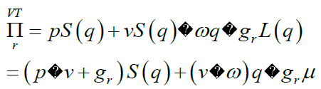
The $\prod_{r}^{V T}(q)$, $\prod_{s}^{V T}(q) and $ VT$ $\Pi$ (q) are used to denote the expected profit of the retailer, the vendor and the entire VMI & TPL supply chain, respectively. The $\prod_{r}^{V T}$, $\prod_{s}^{V T}$ and $ VT$ $\Pi$ are used to denote the profit of the retailer, the profit of the vendor and the profit of the entire VMI & TPL supply chain. In this way, we can obtain the following functions:
The retailer’s profit function:
(8)
The vendor’s profit function:
$\begin{align} & \underset{s}{\overset{VT}{\mathop{\Pi }}}\,=\omega q-{{k}_{2}}cq-{{g}_{s}}L\left( q \right)-f\left( q \right) \\ & =\left( {{g}_{s}}+{{k}_{1}}h \right)S\left( q \right)+\left( \omega -{{k}_{1}}h-{{k}_{2}}c-{{T}_{v}} \right)q-{{g}_{s}}\mu -{{T}_{f}} \\ \end{align}$ (9)
The entire supply chain’s profit function:
$\begin{align} & \overset{VT}{\mathop{\Pi }}\,=\left( p+g+{{k}_{1}}h-v \right)S\left( q \right) \\ & +\left( v-{{k}_{1}}h-{{k}_{2}}c-{{T}_{v}} \right)q-g\mu -{{T}_{f}} \\ \end{align}$ (10)
Compare the retailer’s profit and the vendor’s profit under two types of supply chain modes:
${{\Pi }_{r}}=\underset{r}{\overset{VT}{\mathop{\Pi }}}\,-\underset{r}{\overset{R}{\mathop{\Pi }}}\,={{c}_{r}}q+{{h}_{r}}\left[ q-S\left( q \right) \right]>0$ (11)
$\begin{align} & {{\Pi }_{s}}=\underset{s}{\overset{VT}{\mathop{\Pi }}}\,-\underset{s}{\overset{R}{\mathop{\Pi }}}\, \\ & =\left( {{h}_{s}}-{{k}_{1}}h \right)\left[ q-S\left( q \right) \right]+\left( {{c}_{s}}-{{k}_{2}}c \right)q>0 \\ \end{align}$ (12)
It can be seen from formulas (11) & (12) that the VMI & TPL manages to increase both the retailer’s profit and the vendor’s profit.
3.2 Evolutionary game analysis of supply chain coordination
(1) Construction of game model
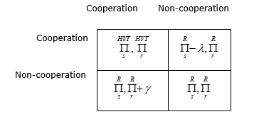
The vendor and the retailer both adopt the strategy set of {cooperation, non-cooperation}, that is, both or neither of the two parties choose cooperation. The situation is called a symmetric game. When both of them choose non-cooperation, the two parties form an RMI supply chain; each of them manages its own inventory and makes its own profit in RMI supply chain. According to the stategy space of VMI & TPL, the TPL participates in the VMI supply chain through transactions. In other words, the TPL only provides services and does not make decisions. Therefore, this paper only considers the strategy selection of the vendor and the retailer. When both of them choose cooperation, the two parties form a VMI & TPL supply chain operation mode with the TPL. Before implementing VMI & TPL supply chain, the two parties need to carry out preliminary works like infrastructure construction, system upgrade and mode optimization. If one of the parties scraps the contract unilaterally, the preliminary investment of the other party will become sunk cost. The profit of the other party is determined by substracting the sunk cost from its profit under RMI supply chain, while the cost of the breaching party is equal to its cost under RMI supply chain. Suppose the preliminary cost of the vendor is m, and that of the retauker is n. Based on the above analysis, the payoff matrix of the retailer and the vendor is obtained (Figure 1).
As analyzed above, the game model is a symmetrical dual population evolutionary game. The evolutionary stability of the vendor and the retailer’s behavior and strategy is analyzed by iterative dynamic equation.
Due to the stochastic and independent nature of the vendor and the retailer’s selection of behavior strategy, the probabilities for the vendor to choose cooperation and non-cooperation are assumed to be a and 1-a, respectively; the probabilities for the retailer to choose cooperation and non-cooperation are assumed to be b and 1- b. Both a and b fall in the range of (0, 1).
$\prod_{s}^{\overline{VT}}$, $\prod_{s}^{\overline{R}}$ and $\overline{\Pi_{s}}$ are used to denote the fitness of the vendor under VMI & TPL strategy, the fitness of the vendor under RML strategy and the average fitness of the vendor, respectively. Then, we have:
$\overline{\underset{s}{\overset{VT}{\mathop{\Pi }}}\,}=\beta \underset{s}{\overset{VT}{\mathop{\Pi }}}\,+\left( 1-\beta \right)\left( \underset{s}{\overset{R}{\mathop{\Pi }}}\,-m \right)$ (13)
$\overline{\underset{s}{\overset{R}{\mathop{\Pi }}}\,}=\beta \underset{s}{\overset{R}{\mathop{\Pi }}}\,+\left( 1-\beta \right)\underset{s}{\overset{R}{\mathop{\Pi }}}\,=\underset{s}{\overset{R}{\mathop{\Pi }}}\,$ (14)
$\overline{{{\Pi }_{s}}}=\alpha \overline{\underset{s}{\overset{VT}{\mathop{\Pi }}}\,}+\left( 1-\alpha \right)\overline{\underset{s}{\overset{R}{\mathop{\Pi }}}\,}$ (15)
By definition, the iterative dynamic equation reflects the direction and the speed of players. The growth rate of the times that the vendor chooses cooperation a*/a is calculated by subtracting the average fitness $\overline{\Pi_{s}}$ from its fitness $\prod_{s}^{\overline{VT}}$. According to formulas (13), (14) & (15), we can get the iterative dynamic equation for the case that the vendor chooses to implement VML & TPL supply chain is:
${}^{{{\alpha }^{*}}}/{}_{\alpha }=\overline{\underset{s}{\overset{VT}{\mathop{\Pi }}}\,}-\overline{{{\Pi }_{s}}}=\left( 1-\alpha \right)\left[ \beta \left( \underset{s}{\overset{VT}{\mathop{\Pi }}}\,-\underset{s}{\overset{R}{\mathop{\Pi }}}\,+m \right)-m \right]$ (16)
Similarly, if the retailer chooses cooperation, its iterative dynamic equation under VML & TPL supply chain is:
${}^{{{\beta }^{*}}}/{}_{\beta }=\overline{\underset{r}{\overset{VT}{\mathop{\Pi }}}\,}-\overline{{{\Pi }_{r}}}=\left( 1-\beta \right)\left[ \alpha \left( \underset{r}{\overset{VT}{\mathop{\Pi }}}\,-\underset{r}{\overset{R}{\mathop{\Pi }}}\,+n \right)-n \right]$ (17)
Let a*=da/dt=0, b *=db/dt=0, and calculate formulas (16) & (17) to get the following conclusion: Conclusion 1: Since a=0.1 and b=0.1, (0, 0), (0, 1), (1, 0), (1, 1) are the evolutionary balance points of VMI & TPL supply chain. If a¹0 or 1 and b¹0 or 1, then:
${{\alpha }_{0}}=\frac{n}{\underset{r}{\overset{VT}{\mathop{\Pi }}}\,-\underset{r}{\overset{R}{\mathop{\Pi }}}\,+n}$ (18)
${{\beta }_{0}}=\frac{m}{\underset{s}{\overset{VT}{\mathop{\Pi }}}\,-\underset{s}{\overset{R}{\mathop{\Pi }}}\,+m}$ (19)
whereas a, bÎ(0, 1), (a0, b0) is also the evolutionary balance point of the supply chain under the condition that a0Î(0, 1), b0Î(0, 1).
For further study on the stability of the evolutionary balance points of the supply chain, it is necessary to establish the Jacobian matrix J:
$\begin{align} & J=\left( \begin{matrix} \frac{d{{\alpha }^{*}}}{d\alpha } & \frac{d{{\alpha }^{*}}}{d\beta } \\ \frac{d{{\beta }^{*}}}{d\alpha } & \frac{d{{\beta }^{*}}}{d\beta } \\ \end{matrix} \right) \\ & =\left( \begin{matrix} \left( 1\text{-2}\alpha \right)\left[ \beta \left( \underset{s}{\overset{VT}{\mathop{\Pi }}}\,-\underset{s}{\overset{R}{\mathop{\Pi }}}\,+m \right)-m \right] & \alpha \left( \text{1-}\alpha \right)\left( \underset{s}{\overset{VT}{\mathop{\Pi }}}\,-\underset{s}{\overset{R}{\mathop{\Pi }}}\,+m \right) \\ \beta \left( 1-\beta \right)\left( \underset{r}{\overset{VT}{\mathop{\Pi }}}\,-\underset{r}{\overset{R}{\mathop{\Pi }}}\,+n \right) & \left( 1-2\beta \right)\left[ \alpha \left( \underset{r}{\overset{VT}{\mathop{\Pi }}}\,-\underset{r}{\overset{R}{\mathop{\Pi }}}\,+n \right)-n \right] \\ \end{matrix} \right) \\ \end{align}$ (20)
The determinant of matrix J is calculated as:
$\begin{align} & J=\left( 1\text{-2}\alpha \right)\left[ \beta \left( \underset{s}{\overset{VT}{\mathop{\Pi }}}\,-\underset{s}{\overset{R}{\mathop{\Pi }}}\,+m \right)-m \right]\cdot \left( 1-2\beta \right)\left[ \alpha \left( \underset{r}{\overset{VT}{\mathop{\Pi }}}\,-\underset{r}{\overset{R}{\mathop{\Pi }}}\,+n \right)-n \right] \\ & -\alpha \left( \text{1-}\alpha \right)\left( \underset{s}{\overset{VT}{\mathop{\Pi }}}\,-\underset{s}{\overset{R}{\mathop{\Pi }}}\,+m \right)\cdot \beta \left( 1-\beta \right)\left( \underset{r}{\overset{VT}{\mathop{\Pi }}}\,-\underset{r}{\overset{R}{\mathop{\Pi }}}\,+n \right) \end{align}$ (21)
The trace value of matrix J stands at:
$\begin{align} & trJ=\left( 1\text{-2}\alpha \right)\left[ \beta \left( \underset{s}{\overset{VT}{\mathop{\Pi }}}\,-\underset{s}{\overset{R}{\mathop{\Pi }}}\,+m \right)-m \right] \\ & \cdot \left( 1-2\beta \right)\left[ \alpha \left( \underset{r}{\overset{VT}{\mathop{\Pi }}}\,-\underset{r}{\overset{R}{\mathop{\Pi }}}\,+n \right)-n \right] \\ \end{align}$ (22)
Figure 1. The payoff matrix of the retailer and the vendor
(2) Solution for the evolutionary stable strategy (ESS) of VMI & TPL supply chain
According to formulas (11) & (12), there are $\prod_{s}^{V T}>\prod_{s}^{R}$ and $\prod_{r}^{V T}>\prod_{r}^{R}$ under the VMI & TPL supply chain. Thus, we can obtain the following formulas:
${{\alpha }_{0}}=\frac{n}{\underset{r}{\overset{VT}{\mathop{\Pi }}}\,-\underset{r}{\overset{R}{\mathop{\Pi }}}\,+n}\in \left( 0,1 \right)$ (23)
${{\beta }_{0}}=\frac{m}{\underset{s}{\overset{VT}{\mathop{\Pi }}}\,-\underset{s}{\overset{R}{\mathop{\Pi }}}\,+m}\in \left( 0,1 \right)$ (24)
As can be seen from conclusion 1, the evolutionary balance points of ESS under the VMI & TPL supply chain include (0, 0), (0, 1), (1, 0), (1, 1) and (a0, b0).
The ESS analysis results of the evolutionary balance points are shown in Table 1.
Table 1. The ESS analysis of VMI & TPL supply chain
|
Evolutionary balance points |
(0, 0) |
(0, 1) |
(1, 0) |
(1, 1) |
\[\left( \frac{n}{\underset{r}{\overset{VT}{\mathop{\Pi }}}\,-\underset{r}{\overset{R}{\mathop{\Pi }}}\,+n},\frac{m}{\underset{s}{\overset{VT}{\mathop{\Pi }}}\,-\underset{s}{\overset{R}{\mathop{\Pi }}}\,+m} \right)\] |
|
|
detJ |
Formula |
mn |
$n\left( \underset{s}{\overset{VT}{\mathop{\Pi }}}\,-\underset{s}{\overset{R}{\mathop{\Pi }}}\, \right)$ |
$m\left( \underset{r}{\overset{VT}{\mathop{\Pi }}}\,-\underset{r}{\overset{R}{\mathop{\Pi }}}\, \right)$ |
$\left( \underset{s}{\overset{VT}{\mathop{\Pi }}}\,-\underset{S}{\overset{R}{\mathop{\Pi }}}\, \right)\left( \underset{r}{\overset{VT}{\mathop{\Pi }}}\,-\underset{r}{\overset{R}{\mathop{\Pi }}}\, \right)$ |
$\frac{-mn\left( \underset{s}{\overset{VT}{\mathop{\Pi }}}\,-\underset{s}{\overset{R}{\mathop{\Pi }}}\, \right)\left( \underset{r}{\overset{VT}{\mathop{\Pi }}}\,-\underset{r}{\overset{R}{\mathop{\Pi }}}\, \right)}{\left( \underset{s}{\overset{VT}{\mathop{\Pi }}}\,-\underset{s}{\overset{R}{\mathop{\Pi }}}\,+m \right)\left( \underset{r}{\overset{VT}{\mathop{\Pi }}}\,-\underset{r}{\overset{R}{\mathop{\Pi }}}\,+n \right)}$ |
|
Symbol |
+ |
+ |
+ |
+ |
- |
|
|
trJ |
Formula |
-m-n |
$\underset{s}{\overset{VT}{\mathop{\Pi }}}\,-\underset{s}{\overset{R}{\mathop{\Pi }}}\,+n$ |
$\underset{r}{\overset{vt}{\mathop{\Pi }}}\,-\underset{r}{\overset{R}{\mathop{\Pi }}}\,+m$ |
$-\left( \underset{s}{\overset{VT}{\mathop{\Pi }}}\,-\underset{s}{\overset{R}{\mathop{\Pi }}}\, \right)-\left( \underset{r}{\overset{VT}{\mathop{\Pi }}}\,-\underset{r}{\overset{R}{\mathop{\Pi }}}\, \right)$ |
0 |
|
Symbol |
- |
+ |
+ |
- |
|
|
|
Equilibrium outcomes |
ESS |
Unstable point |
Unstable point |
ESS |
Saddle Point |
|
In order to overcome the coordination instability in the VMI & TPL supply chain, this paper introduces the buyback contract to improve the original supply chain. Thus, the strategy space of each node enterprise in the supply chain is changed into: The retailer selects the nearest warehouse, the vendor determines the inventory, and the TPL, only responsible for the establishment of information platform, inventory management, and products delivery, receives the commission from the vendor according to the service it has provided. The ownership of inventory will be transferred to retailer after the TPL completes products delivery. However, under the conditions of excess inventory or direct selling, the retailer is allowed to return the products but should give a partial refund to the vendor.
4.1 Profit analysis of the supply chain
The vendor’s buyback price per unit product is denoted as b, and the buyback contract is described by {w, b}. For the sake of generality, it is assumed that: v<b<cs<w<p, and the retailer cannot get profit from unsold products. Thus, b+v<w and the transfer payment is: Tb(q, w, b)=wq-bI(q)=bs(q)-(w-b)q.
$\prod_{r}^{HVT}$, $\prod_{s}^{HVT}$ and $\underset{{}}{\overset{HVT}{\mathop{\Pi }}}\,$ are used to denote represent the profit of the retailer, the vendor and the entire VMI & TPL supply chain after introducing the buyback contract, respectively. In this way, we can obtain the following functions:
The retailer’s profit function:
$\begin{align} & \underset{r}{\overset{HVT}{\mathop{\prod }}}\,=pS\left( q \right)-T\left( q,w,b \right)-{{g}_{r}}L\left( q \right) \\ & =\left( p-b+{{g}_{r}} \right)S\left( q \right)-\left( w-b \right)q-{{g}_{r}}\mu \\ \end{align}$ (25)
The vendor’s profit function:
$\begin{align} & \underset{s}{\overset{HVT}{\mathop{\prod }}}\,=T\left( q,w,b \right)+vI\left( q \right)-{{k}_{2}}cq-{{g}_{s}}L\left( q \right)-f\left( q \right) \\ & =\left( b+{{g}_{s}}+{{k}_{1}}h-v \right)S\left( q \right) \\ & +\left( w+v-b-{{k}_{2}}c-{{T}_{v}}-{{k}_{1}}h \right)q-{{g}_{s}}\mu -{{T}_{f}} \\ \end{align}$(26)
The entire supply chain’s profit function:
$\begin{align} & \overset{HVT}{\mathop{\prod }}\,=\underset{r}{\overset{HVT}{\mathop{\Pi }}}\,+\underset{s}{\overset{HVT}{\mathop{\Pi }}}\,=pS\left( q \right)+vI\left( q \right)-cq-gL\left( q \right)-f\left( q \right) \\ & =\left( p+g+{{k}_{1}}h-v \right)S\left( q \right)-\left( {{k}_{2}}c-v+{{T}_{v}}+{{k}_{1}}h \right)q-g\mu -{{T}_{f}} \\ \end{align}$ (27)
According to formulas (4), (5), (25) & (26), we can obtain the following:
$\underset{r}{\overset{HVT}{\mathop{\Pi }}}\,-\underset{r}{\overset{R}{\mathop{\Pi }}}\,=\left( b+{{h}_{r}}-v \right)\left[ q-S\left( q \right) \right]>0$ (28)
$\begin{align} & \underset{s}{\overset{HVT}{\mathop{\Pi }}}\,-\underset{s}{\overset{R}{\mathop{\Pi }}}\,=\left( {{k}_{1}}h-{{h}_{s}} \right)S\left( q \right) \\ & +\left( {{c}_{s}}-{{k}_{2}}c+{{h}_{s}}-{{k}_{1}}h \right)q-\left( b-v \right)\left[ q-S\left( q \right) \right] \\ \end{align}$(29)
From the assumptions, it can be deducted that $\left( {{k}_{1}}h-{{h}_{s}} \right)S\left( q \right)>0$, $\left( {{c}_{s}}-{{k}_{2}}c+{{h}_{s}}-{{k}_{1}}h \right)q>0$ and $\left( b-v \right)\left[ q-S\left( q \right) \right]<0$ in formula (29). According to the operation mode of VMI & TPL supply chain, the supply-demand information is updated in real-time owing to the professional information system and strong information processing ability of the TPL. Therefore, the cost reduction through the introduction of TPL and VMI far exceeds the vendor’s profit loss caused by information delay, i.e.
$\underset{s}{\overset{HVT}{\mathop{\Pi }}}\,-\underset{s}{\overset{R}{\mathop{\Pi }}}\,>0$. Compared to RMI mode, the vendor’s profit and the retailer’s profit have been substantially improved after introducing the buyback contract to VMI & TPL supply chain.
4.2 Evolutionary game analysis of supply chain coordination
(1) Construction of game model
Comparing formula (4) with formula (25), we can get:
$\underset{r}{\overset{HVT}{\mathop{\Pi }}}\,-\underset{r}{\overset{HR}{\mathop{\Pi }}}\,=\left( b-v \right)\left[ q-S\left( q \right) \right]>0$ (30)
Comparing formula (5) with formula (26), we can get:
$\underset{s}{\overset{HVT}{\mathop{\Pi }}}\,-\underset{s}{\overset{HR}{\mathop{\Pi }}}\,=-\left( b-v \right)\left[ q-S\left( q \right) \right]<0$ (31)
According to formulas (30) & (31), the supply chain profit is redistributed between the vendor and the retailer after introducing the buyback contract to the VMI & TPL supply chain. When the vendor chooses cooperation and the retailer chooses non-cooperation, the vendor’s payoff function is $\underset{s}{\overset{R}{\mathop{\Pi }}}\,-m-\left( b-v \right)\left[ q-S\left( q \right) \right]$; when the retailer chooses cooperation and the vendor chooses non-cooperation, the retailer’s payoff function is $\underset{r}{\overset{R}{\mathop{\Pi }}}\,-n+\left( b-v \right)\left[ q-S\left( q \right) \right]$.
$\lambda =m+\left( b-v \right)\left[ q-S\left( q \right) \right]$ (32)
$\gamma =\left( b-v \right)\left[ q-S\left( q \right) \right]\text{-}n$ (33)
During repeated game, the retailer’s initial cost is fixed, while the extra profit in formula (30) is cumulative. The extra profit will accumulate as long as the buyback contract exists. Thus, the final evolution result is g>0.
Based on the above analysis, the payoff matrix of the retailer and the vendor in the VMI & TPL after introducing buyback contract (Figure 2).
Figure 2. The payoff matrix of the retailer and the vendor under the buyback contract
(2) Solution for the ESS of VMI & TPL supply chain after introducing buyback contract
According to the above payoff matrix, the vendor’s iterative dynamic equation is:
${}^{{{\alpha }^{*}}}/{}_{\alpha }=\overline{\underset{s}{\overset{HVT}{\mathop{\Pi }}}\,}-\overline{{{\Pi }_{s}}}=\left( 1-\alpha \right)\left[ \beta \left( \underset{s}{\overset{HVT}{\mathop{\Pi }}}\,-\underset{s}{\overset{R}{\mathop{\Pi }}}\,+\lambda \right)-\lambda \right]$ (34)
The retailer’s iterative dynamic equation is:
${}^{{{\beta }^{*}}}/{}_{\beta }=\overline{\underset{r}{\overset{HVT}{\mathop{\Pi }}}\,}-\overline{{{\Pi }_{r}}}=\left( 1-\beta \right)\left[ \alpha \left( \underset{r}{\overset{HVT}{\mathop{\Pi }}}\,-\underset{r}{\overset{R}{\mathop{\Pi }}}\,\text{-}\gamma \right)+\gamma \right]$ (35)
The evolutionary balance points of the supply chain after introducing buyback contract are obtained by formulas (30) & (31):
${{\alpha }_{0}}=\frac{-\gamma }{\underset{r}{\overset{HVT}{\mathop{\Pi }}}\,-\underset{r}{\overset{R}{\mathop{\Pi }}}\,-\gamma }=\frac{-\gamma }{{{h}_{r}}\left[ q-S\left( q \right) \right]+n}<0$ (36)
That is:
${{\alpha }_{0}}\notin \left( 0,1 \right) {{\beta }_{0}}=\frac{\lambda }{\underset{s}{\overset{HVT}{\mathop{\Pi }}}\,-\underset{s}{\overset{R}{\mathop{\Pi }}}\,+\lambda }$ (37)
This means b0Î(0, 1), and thus excludes (a0, b0) from the set of evolutionary balance points. Therefore, the evolutionary balance points of the supply chain after introducing buyback contracts include (0, 0), (0, 1), (1, 0), (1, 1).
The Jacobian matrix J’ if the new supply chain system is established as:
$\begin{align} & {{J}^{'}}=\left( \begin{matrix} \frac{d{{\alpha }^{*}}}{d\alpha } & \frac{d{{\alpha }^{*}}}{d\beta } \\ \frac{d{{\beta }^{*}}}{d\alpha } & \frac{d{{\beta }^{*}}}{d\beta } \\ \end{matrix} \right) \\ & =\left( \begin{matrix} \left( 1\text{-2}\alpha \right)\left[ \beta \left( \underset{s}{\overset{HVT}{\mathop{\Pi }}}\,-\underset{s}{\overset{R}{\mathop{\Pi }}}\,+\lambda \right)-\lambda \right] & \alpha \left( \text{1-}\alpha \right)\left( \underset{s}{\overset{HVT}{\mathop{\Pi }}}\,-\underset{s}{\overset{R}{\mathop{\Pi }}}\,+\lambda \right) \\ \beta \left( 1-\beta \right)\left( \underset{r}{\overset{HVT}{\mathop{\Pi }}}\,-\underset{r}{\overset{R}{\mathop{\Pi }}}\,-\gamma \right) & \left( 1-2\beta \right)\left[ \alpha \left( \underset{r}{\overset{HVT}{\mathop{\Pi }}}\,-\underset{r}{\overset{R}{\mathop{\Pi }}}\,-\gamma \right)+\gamma \right] \\ \end{matrix} \right) \\ \end{align}$ (38)
The determinant of matrix J’ is calculated as:
$\begin{align} & {{J}^{'}}=\left( 1\text{-2}\alpha \right)\left[ \beta \left( \underset{s}{\overset{HVT}{\mathop{\Pi }}}\,-\underset{s}{\overset{R}{\mathop{\Pi }}}\,+\lambda \right)-\lambda \right]\cdot \left( 1-2\beta \right)\left[ \alpha \left( \underset{r}{\overset{HVT}{\mathop{\Pi }}}\,-\underset{r}{\overset{R}{\mathop{\Pi }}}\,-\gamma \right)+\gamma \right] \\ & -\alpha \left( \text{1-}\alpha \right)\left( \underset{s}{\overset{HVT}{\mathop{\Pi }}}\,-\underset{s}{\overset{R}{\mathop{\Pi }}}\,+\lambda \right)\cdot \beta \left( 1-\beta \right)\left( \underset{r}{\overset{HVT}{\mathop{\Pi }}}\,-\underset{r}{\overset{R}{\mathop{\Pi }}}\,-\gamma \right) \\ \end{align}$ (39)
The trace value of matrix J’ stands at:
$\begin{align} & tr{{J}^{'}}=\left( 1\text{-2}\alpha \right)\left[ \beta \left( \underset{s}{\overset{HVT}{\mathop{\Pi }}}\,-\underset{s}{\overset{R}{\mathop{\Pi }}}\,+\lambda \right)-\lambda \right] \\ & \cdot \left( 1-2\beta \right)\left[ \alpha \left( \underset{r}{\overset{HVT}{\mathop{\Pi }}}\,-\underset{r}{\overset{R}{\mathop{\Pi }}}\,-\gamma \right)+\gamma \right] \\ \end{align}$(40)
The ESS analysis results of the evolutionary balance points are shown in Table 2.
Table 2. The ESS analysis of VMI & TPL supply chain after introducing buyback contract
|
Evolutionary balance points |
(0, 0) |
(0, 1) |
(1, 0) |
(1, 1) |
|
|
detJ |
Formula |
$\text{-}\lambda \gamma $ |
$-\gamma \left( \underset{s}{\overset{HVT}{\mathop{\Pi }}}\,-\underset{s}{\overset{R}{\mathop{\Pi }}}\, \right)$ |
$\lambda \left( \underset{r}{\overset{HVT}{\mathop{\Pi }}}\,-\underset{r}{\overset{R}{\mathop{\Pi }}}\, \right)$ |
$\left( \underset{s}{\overset{HVT}{\mathop{\Pi }}}\,-\underset{S}{\overset{R}{\mathop{\Pi }}}\, \right)\left( \underset{r}{\overset{HVT}{\mathop{\Pi }}}\,-\underset{r}{\overset{R}{\mathop{\Pi }}}\, \right)$ |
|
Symbol |
- |
- |
+ |
+ |
|
|
trJ |
Formula |
$-\lambda +\gamma $ |
$\underset{s}{\overset{HVT}{\mathop{\Pi }}}\,-\underset{s}{\overset{R}{\mathop{\Pi }}}\,-\gamma $ |
$\underset{r}{\overset{HVT}{\mathop{\Pi }}}\,-\underset{r}{\overset{R}{\mathop{\Pi }}}\,+\lambda $ |
$-\left( \underset{s}{\overset{HVT}{\mathop{\Pi }}}\,-\underset{s}{\overset{R}{\mathop{\Pi }}}\, \right)-\left( \underset{r}{\overset{HVT}{\mathop{\Pi }}}\,-\underset{r}{\overset{R}{\mathop{\Pi }}}\, \right)$ |
|
Symbol |
Adventitious |
Adventitious |
+ |
- |
|
|
Equilibrium outcomes |
Saddle Point |
Saddle Point |
Unstable Point |
ESS |
|
Table 3. The profit comparison between all supply chains modes
|
|
${{\Pi }_{r}}$ |
${{\Pi }_{s}}$ |
$\Pi $ |
|
RMI |
138.17 |
264.11 |
402.28 |
|
VMI & TPL |
443.55 |
599.82 |
1043.37 |
|
VMI & TPI after introducing buyback contract |
451.74 |
591.63 |
1043.37 |
It can be seen from Table 3 that \[\underset{r}{\overset{HVT}{\mathop{\prod }}}\,>\underset{r}{\overset{R}{\mathop{\prod }}}\,\], $\underset{r}{\overset{VT}{\mathop{\Pi }}}\,>\underset{r}{\overset{R}{\mathop{\Pi }}}\,$ and $\underset{\text{s}}{\overset{HVT}{\mathop{\Pi }}}\,>\underset{s}{\overset{R}{\mathop{\Pi }}}\,$, $\underset{s}{\overset{VT}{\mathop{\Pi }}}\,>\underset{s}{\overset{R}{\mathop{\Pi }}}\,$, indicating that the vendor (Company B), the retailer (Company A) and the entire supply chain have made more profit under VMI & TPI and VMI & TPI after introducing buyback contract than under the traditional RMI mode. It can also be inferred that $\underset{r}{\overset{HVT}{\mathop{\Pi }}}\,>\underset{r}{\overset{VT}{\mathop{\Pi }}}\,$, $\underset{\text{s}}{\overset{HYT}{\mathop{\Pi }}}\,<\underset{s}{\overset{VT}{\mathop{\Pi }}}\,$ and $\underset{r}{\overset{HVT}{\mathop{\Pi }}}\,+\underset{s}{\overset{HVT}{\mathop{\Pi }}}\,=\underset{r}{\overset{VT}{\mathop{\Pi }}}\,+\underset{s}{\overset{VT}{\mathop{\Pi }}}\,$, which proves the profit redistribution between the vendor and the retailer after introducing the buyback contract to VMI & TPL although the overall profit of the supply chain remains the same before and after the introduction.
Substitute the results in Table 3 into formulas (17) & (18), we have: ${{\alpha }_{0}}=\frac{\text{n}}{305.38+n}>0$, ${{\beta }_{0}}=\frac{m}{335.71+m}>0$, that is, the evolutionary balance points of the supply chain are (0, 0), (0, 1), (1, 0), (1, 1) and (a0, b0) before introducing the buyback contract. The ESS analysis of each evolutionary balance point is shown in Table 4.
Table 4. The ESS analysis of VMI & TPL supply chain
|
Evolutionary balance points |
(0,0) |
(0,1) |
(1,0) |
(1,1) |
$\left( \frac{\text{n}}{305.38+n},\frac{m}{335.71+m} \right)$ |
|
|
detJ |
Result |
mn |
335.71n |
305.38m |
102519.12 |
$\frac{-102519.12mn}{\left( 305.38+n \right)\left( 335.71+m \right)}$ |
|
Symbol |
+ |
+ |
+ |
+ |
- |
|
|
trJ |
Result |
-m-n |
335.71+n |
305.38+m |
-641.09 |
0 |
|
Symbol |
- |
+ |
+ |
- |
|
|
|
Equilibrium outcomes |
ESS |
Unstable point |
Unstable point |
ESS |
Saddle point |
|
Substitute the results in Table 4 into formulas (36) & (37), we have: a0=-g/(313.57-g), b0=(l/(327.52+l))>0. According to the analysis of formula (36), (a0, b0) is excluded from the set of evolutionary balance points due to the fact that a0<0. That is to say, the evolutionary balance points of the supply chain after introducing buyback contract include (0, 0), (0, 1), (1, 0), (1, 1). The ESS analysis of each evolutionary balance point shows that the value of $\underset{s}{\overset{HVT}{\mathop{\Pi }}}\,-\underset{s}{\overset{R}{\mathop{\Pi }}}\,-\gamma $ changes with the value of $\underset{s}{\overset{HVT}{\mathop{\Pi }}}\,$, making it impossible to determine its positive and negative properties. The results are shown in Table 5.
Table 5. The ESS analysis of VMI & TPI after introducing buyback contract
|
Evolutionary balance points |
(0, 0) |
(0, 1) |
(1, 0) |
(1, 1) |
|
|
detJ |
Result |
-lg |
-327.52$\gamma $ |
313.57$\lambda $ |
102700.45 |
|
Symbol |
- |
- |
+ |
+ |
|
|
trJ |
Result |
-l+g |
327.52-g |
313.57+l |
-641.09 |
|
Symbol |
Adventitious |
Change with $\underset{s}{\overset{HVT}{\mathop{\Pi }}}\,$ value |
+ |
- |
|
|
Equilibrium outcomes |
Saddle Point |
Saddle Point |
Unstable Point |
ESS |
|
This paper applies the evolutionary game analysis method to the research of supply chain coordination, introduces the buyback contract model to the coordination study of VMI & TPL supply chain, and conducts model calculations and case analysis. The conclusions are as follows: the introduction of buyback contract effectively improves the coordination and stability of VMI & TPL supply chain because it transforms the ESS of (cooperation, cooperation) and (non-cooperation, non-cooperation) into (cooperation, cooperation). The improved supply chain can realize stable development in the competitive market. Future research will focus on the construction of a coordination model involving multiple vendors, TPLs and retailers
Thank the National Science Foundation Project: Research on Collaborative Innovation System of the Pearl River-Xijiang River Economic Belt under Supply-side Reform for supporting this research through Grant No.17XGL006, and Wuzhou University Foundation Project: Research on transformation and upgrading of manufacturing industry for the Pearl River-Xijiang River Economic Belt, No. 2017A002.
[1] Cai, J., Huang, W., Zhou, G. (2006). Study on VMI model based on revenus-sharing contract. Chinese Journal of Management Science, 14(4): 108-113.
[2] Wang, W., Zhang J. (2008). A VMI environment coordination contract and its resistance to emergencies. Chinese Journal of Management Science, 16(5): 414-419.
[3] Cachon, G.P. (2001). Stock war: Inventory competition in a two-echelon supply chain with multiple retailers. Operations Research, 49(5): 658-674. https://doi.org/10.1287/opre.49.5.658.10611
[4] Cetinkaya, S., Lee, C.Y. (2000). Stock replenishment and shipment scheduling for vendor-managed inventory systems. Management Science, 46(2): 217-232. https://doi.org/10.1287/mnsc.46.2.217.11923
[5] Achabal, D.D., McIntyre, S.H., Smith, S.A. (2000). A decision support system for vendor managed inventory. Journal of Retailing, 76(4): 430-454. https://doi.org/10.1016/S0022-4359(00)00037-3
[6] Disney, S.M., Towill, D.R. (2003). The effect of vendor managed inventory (VMI) dynamics on the Bullwhip Effect in supply chains. International Journal of Production Economics, 85(2): 199-215. https://doi.org/10.1016/S0925-5273(03)00110-5
[7] Tyan T., Wee, H.M. (2003). Vendor managed inventory a survey of the Taiwanese grocery industry. Journal of Purchasing and Supply Management, 9(1): 11-18. https://doi.org/10.1016/S0969-7012(02)00032-1
[8] Yu, Y., Chu F., Chen H. (2009). A Stackelberg game and its improvement in a VMI system with a manufacturing vendor. European Journal of Operational Research, 192(3): 929-948. https://doi.org/10.1016/j.ejor.2007.10.016
[9] Han, C., Liu, Z. (2011). Integrated model and strategic space of VMI & TPL supply chain. Industrial Engineering and Management, 16(2): 97-102.
[10] Han, C., Liu, Z. (2011). The cooperation mechanism of VMI & TPL apply chain based on evolutionary game. Industrial Engineering and Management, 16(6): 21-29.
[11] Zhang, C., Zhou, Y. (2010). Revenue sharing mechanism coordination model based on game theory and VMI. Control and Decision, 25(1): 137-144.
[12] Jin, C., Cao, E., Lai, M. (2012). Analysis on green marketing strategy of duopoly retailing market based on the evolutionary game theory. Journal of Systems Engineering, 27(3): 383-389.
[13] Huang, M. (2010). The cooperation mechanism of supply chain collaborative product development based on evolutionary game. Chinese Journal of Management Science, 18(6): 155-161.