Huaping Mu
OPEN ACCESS
Aiming at the disturbance event of single machine sudden failure in the initial job scheduling of flexible job shop, the dissatisfaction of customers, enterprises and labor workers is quantified using the unascertained theory, and a scheduling interference management model considering the characteristics of three parties is constructed. The NSGA-II algorithm is improved using the strategy of close relative crossover and mutation, and the efficient solution to the flexible job shop scheduling problem is realized. The example shows that the interference management model proposed in this paper can better reduce disturbance of the disturbance events compared with rescheduling, AOR rescheduling and full right shift scheduling, which can restore the normal operation of the processing and manufacturing system to realize the coordination of different stakeholders.
flexible job-shop scheduling, close relative crossover and mutation, NSGA-II; multi-objective optimization, behavior perception
In the multispecies and middle and small batch customized production mode, the balance between production plan and operation plan is easy to be disturbed, and the original production scheduling plan cannot be implemented normally [1]. Flexible job shop scheduling problem (FJSP) is an extension of job shop scheduling problem (JSP), which reduces machine constraints, makes the search for feasible solutions more difficult [2], and is more in line with the scheduling practice of advanced manufacturing enterprises under the JIT thought. However, the flexible job shop scheduling is a typical human-machine synergy system, which combines the participants of the scheduling with the resource scheduling in the traditional operation management. The factors of people mainly include customers, manufacturers and workers in workshops, which have been paid more and more attention in reality [3]. At the same time, the production process is more susceptible to some interference events, such as machine failure, order production adjustment, process delay, raw material supply interruption, and so on, so that the initial scheduling plan cannot be implemented smoothly [4, 5].
The research on the problem of workshop scheduling interference is mainly focused on single machine, parallel machine, flow shop, job shop and open workshop environment. The classical job shop scheduling methods mainly include rescheduling [6], robust scheduling [7, 8], rightward shift scheduling [9] and AOR rescheduling [10, 11]. These methods can adjust the scheduling plan and enrich the job shop scheduling method. The interference management is not to optimize the state of the disturbance after the occurrence of the disturbance. By optimizing the initial scheme, the disruption management scheduling scheme is quickly generated which has the minimum disturbance effect on the system. Ding [12] used local rescheduling to deal with the interruption of all machine processing in the initial scheduling of JSP environment. Jiang [13] and Liu [6] dealt with interference events in single machine shop environment using lexicographical order multi-objective programming and rescheduling. Ayten et al. [14] realized disturbance measurement using integer programming method in parallel machine environment. Louis and Xu [15] dealt with the problem of machine fault interference and update interference in an open workshop using the rescheduling strategy of genetic algorithm. Aiming at the new workpiece arrival interference in job shop scheduling, Wang [16] and Wang [17] adopted the hybrid evolutionary algorithm of rescheduling and meta heuristic to deal with the interference.
The modeling method of job shop scheduling interference considering behavior is mainly based on the prospect theory and fuzzy mathematics. On the basis of prospect theory and fuzzy mathematics, the “limited rationality” of human is extracted. Ding [12] and Jiang [13] set up a lexicographical order multi-objective interference management model. Wang [17] established an interference management model considering the initial cost target and the disturbance target.
The solution of FJSP is mainly sought using the genetic algorithm and the non-dominated sorting algorithm. Chen et al. [18] proposed a hybrid genetic algorithm with bottlenecks, Chen [19] proposed a NSGA- II algorithm based on the variation of close relatives, and Wu [20], Wei [21] used the improved genetic algorithm to solve the flexible job shop scheduling problem.
At present, different types of job shop scheduling interference problems have been preliminarily studied, but researches on more complex job shop interference problems have not started yet. The measurement of the behavior perception of behavioral agent are mainly conducted using fuzzy mathematics and the diversified dissatisfaction measurement tools are lacking. Although NSGA-II is the mainstream algorithm for solving multi-objective optimization problems, it is easy to fall into local convergence.
Based on the above analysis, in this paper, under the flexible job shop environment, the single machine fault interference occurs during the initial scheduling execution process, and multi-agent behavior perception is considered. The unascertained theory is used to measure the dissatisfaction of different stakeholders, and the model of interference management is set up. The improved NSGA-II algorithm based on close relative crossover and mutation is applied to enhance the local search ability of the algorithm, and the elitist strategy is adopted to accelerate the optimization speed and finally the Pareto optimal solution set is obtained. Then, according to the importance of different stakeholders, the optimal solution of single machine fault FJSP is found.
Every process in FJSP can be processed on different machines. It mainly includes two questions: determining the processing machines for each part of the work-piece, and determining the processing sequence of each process on each machine [19]. During the execution of the initial scheduling plan, a machine suddenly fails and needs to be repaired for continuous use. The interference events make the original scheduling unable to continue, and interference treatment is needed. Rescheduling will increase the workload of repetitive handling, clamping and coordination, which directly causes workers’ dissatisfaction to increase. The delayed deliveries of the workpiece will lead to dissatisfaction of the customer and the manufacturer. The interference management should start from the overall interests of the manufacturing system and minimize the dissatisfaction of the interference events to the whole manufacturing system.
Rescheduling after disturbances in flexible job shop scheduling will inevitably change the original scheduling plan, resulting in the tardiness of workpiece and the change of workpiece processing sequence and dissatisfaction of customers, manufacturers and workshop workers. People are in an irrational state [22], and the dissatisfaction of these agents in the job shop scheduling system will restrict the operation efficiency of the supply chain, or even lead to the breakdown of the cooperative relationship, which is also the key to the effective implementation of the shop scheduling theory in the actual production.
The prospect theory, based on the limited rationality of human, can describe the people’s behavior preference under different circumstances. The value function of the subject of behavior can be expressed as Eq. (1):
$V_{r}(x)=\left\{\begin{array}{c}{x^{\alpha_{r}}, x \geq 0} \\ {-\lambda_{r}(-x)^{\beta_{r}}, x<0}\end{array}\right.$ (1)
where, $x=\frac{x_{i}-x_{0}}{l}$, l is the maximum perturbation value, $l_{r}=\max \left(x_{i}-x_{0}\right), i=1,2, \ldots, n, x_{0}$, is the reference point, that is the minimum value of the behavior subject affected by the interference factor. $\alpha, \beta$ are the risk attitude coefficients, $a_{r}>0,0<\beta_{r}<1 . \lambda$ is the loss aversion coefficient, $\lambda>1$.
If the interference of machine failure occurs in the processing of the workshops, the losses to the manufacturers, customers and workshops are mainly reflected in the part of $x_{i}<O_{i}$. The value function can be transformed into Eq. (2) through deformation.
$\mu\left(x_{i}\right)=-V(-x)=\lambda_{r}\left(\frac{x_{i}-x_{0}}{l_{r}}\right)^{\beta_{r}}$ (2)
The unascertained theory is different from the theory of random and fuzzy [23, 24], which can judge and quantify items [25] in the case of incomplete information according to the prior knowledge. Unascertained mathematical theory has been widely used in economy, engineering, enterprise management, environmental evaluation and so on. Using unascertained mathematics to measure the dissatisfaction of the behavior subject, we can get the membership function of the dissatisfaction measure of the behavior subject.
3.1 Subordination function of dissatisfaction measure of different behavior subjects
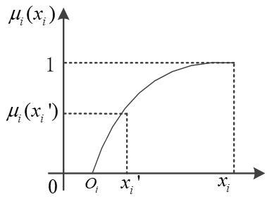
According to the unascertained mathematics, the degree of dissatisfaction of behavioral subjects in the sense of unstrict measurement are measured, and the unascertained measure function $\mu_{r}$ of different behavior subjects based on prospect theory is constructed. The disturbance loss of different behavior subjects is transformed into the number between 0-1 by using the unascertained degree of membership. It shows the dissatisfaction of different agents. 1 indicates that the behavior subject is not satisfied, 0 indicates that the subject is satisfied. The dissatisfaction of the behavioral subject r to the evaluation object i is $\mu_{r}\left(x_{i}\right)$, and the subjection function of the dissatisfaction measure of the behavior subject is as follows Eq. (3), $R_{i}^{r}=t_{0}+l\left(\frac{1}{\lambda_{r}}\right)^{\frac{1}{\beta_{r}}}$. The measure function of the dissatisfaction of the behavior subject is shown in Figure 1.
$\mu_{r}(x)=\lambda_{r}\left(\frac{x_{i}-x_{0}}{l_{r}}\right)^{\beta_{r}}, x_{0} \leq x_{i} \leq R_{i}^{r}$ (3)
Figure 1. The subjection function of the dissatisfaction measure of the behavior subject
(1) The customer’s dissatisfaction is mainly determined by the tardiness of the work piece. The maximum tardiness time of the work-piece $l=\max \left(t_{i}-t_{i}^{0}\right), i=1,2, \ldots, n$. The completion time of the workpiece is $t_{i}$. $t_{i}^{0}$ is the original scheduling completion time of the workpiece i. Customer’s dissatisfaction with the scheduling is $\mu_{1}$. The measure of the customer’s dissatisfaction with the workpiece i is as follows:
$\mu_{1}^{\prime}\left(t_{i}\right)=\left\{\begin{array}{c}{1, \quad t_{i} \geq R_{i}^{1}} \\ {\lambda_{1}\left(\frac{t_{i}-t_{i}^{0}}{l}\right)^{\beta_{1}}, \quad t_{i}^{0} \leq t_{i}<R_{i}^{1}} \\ {0, \quad t_{i}<t_{i}^{0}}\end{array}\right.$ (4)
where, $R_{i}^{1}=t_{i}^{0}+l\left(\frac{1}{\lambda_{1}}\right)^{\frac{1}{\beta_{1}}}, \mu_{1}(t)=\frac{\sum_{i=1}^{n} \mu_{1}^{\prime}\left(x_{i}\right)}{n}$.
(2) The dissatisfaction of manufacturer is mainly influenced by the completion time of the work piece. The completion time of the original scheduling is $t_{0}$, and the average tardiness time of the new scheduling is $\Delta t=\frac{\sum_{i=1}^{n}\left(t_{i}-t_{i}^{0}\right)}{n}$. The manufacturer’s dissatisfaction measure is as follows:
$\mu_{2}(t)=\left\{\begin{array}{c}{1, \Delta t \geq R_{i}^{2}} \\ {\lambda_{2}\left(\frac{\Delta t}{l}\right)^{\beta_{2}}, \quad 0 \leq \Delta t<R_{i}^{2}}\end{array}\right.$ (5)
where, $R_{i}^{2}=l\left(\frac{1}{\lambda_{2}}\right)^{\frac{1}{\beta_{2}}}$.
(3) The dissatisfaction of the working workers in the workshop is mainly caused by the complex workshops. Employees are most concerned about the changes in the number of work-pieces on each machine in the new and old scheduling, that is, the number of disturbance processes. For example, the original machine 1, the need to carry 3 pieces of jobs, after the rescheduling of the need to carry 4 pieces of jobs, the number of disturbances on this machine is 1. The sum of the disturbances on all machines is the total number of perturbations $n_{a f f c e t e d}, n_{s u m}$ is the total number of processes.
$\mu_{3}\left(n_{a f f c e t e d}\right)=\left\{\begin{array}{c}{1, n_{a f f c e t e d} \geq R_{i}^{3}} \\ {\lambda_{3}\left(\frac{n_{a f f c e t e d}}{n_{s u m}}\right)^{\beta_{3}}, 0 \leq n_{a f f c e t e d}<R_{i}^{3}}\end{array}\right.$ (6)
where, $R_{i}^{3}=n_{\operatorname{sum}}\left(\frac{1}{\lambda_{3}}\right)^{\frac{1}{\beta_{3}}}$.
3.2 Construction of interference management model
(1) Parameter and Variable Description
n: Total number of pieces;
m: Total number of machines;
i: Machine serial number, $i=1,2,3, \dots, m$;
j,k: Work-piece sequence number, $j, k=1,2,3, \dots n$;
$h_{j}$: The total number of processes for the jth work piece, $h=1,2,3, \ldots, h_{j}$;
l: Working procedure serial number, $l=1,2,3, \ldots, h_{j}$;
$m_{j h}$: The number of optional processing machines in the hth process of the jth work piece;
$O_{j h}$: The hth process of the jth workpiece;
$M_{i j h}$: The hth process of the jth work-piece is processed on the machine i;
$p_{i j k}$: The processing time of the hth working procedure of the jth workpiece on the machine i;
$S_{j h}$: The time for the starting process of the hth process of the jth work piece;
$C_{j h}$: The processing completion time of the hth process of the jth work piece;
L: A enough large number;
$C_{j}$: The completion time of the workpiece j;
$C_{\max }$: The maximum completion time;
(2) Interference Management Model
$\min f_{1}=\mu_{1}(t)$ (7)
$\min f_{2}=\mu_{2}(t)$ (8)
$\min f_{3}=\mu_{3}\left(n_{a f f e c t e d}\right)$ (9)
s.t. $\quad s_{j h}+x_{i j h} p_{i j k} \leq c_{j h}$ (10)
$s_{j k}+x_{i j h} p_{i j h} \leq c_{j h},$ where $h=1,2,3, \dots, h_{j-1}$ (11)
$c_{j h} \leq S_{j(h+1)}$ (12)
$s_{j h}+p_{i j h} \leq s_{k l}+L\left(1-y_{i j h k l}\right)$ (13)
$c_{j h} \leq s_{j(h+1)}+L\left(1-y_{i k l j(h+1)}\right)$ (14)
$\sum_{i=1}^{m_{i h}} x_{i j h}=1$ (15)
$\sum_{j=1}^{n} \sum_{h=1}^{h_{j}} y_{i j h k l}=x_{i k l}$ (16)
$\sum_{k=1}^{n} \sum_{l=1}^{h_{k}} y_{i j h k l}=x_{i j h}$ (17)
$s_{i h} \geq 0, c_{j h} \geq 0$ (18)
where, $x_{i j h}=1$, if the procedure $O_{j h}$ is finished on machine i; otherwise, $x_{i j h}=0$. $y_{i j h k l}=1$, if the procedure $O_{i j h}$ is finished before the procedure $O_{i k l}$, otherwise it is 0.
Eq. (7), (8) and (9) are the objective functions to express the dissatisfaction of the customers, the manufacturers and the labour workers of the workshops. Eq. (10) and (11) represent the process constraints to the workpiece. Eq. (12) indicates that a work procedure cannot be processed until the last work procedure is completed. Eq. (13) and (14) indicate that one machine can only process one workpiece at the same time. Eq. (15), (16) and (17) represent a machine repeatedly operates each working procedure. Eq. (18) indicates that the processing cannot be started until the workpiece arrives.
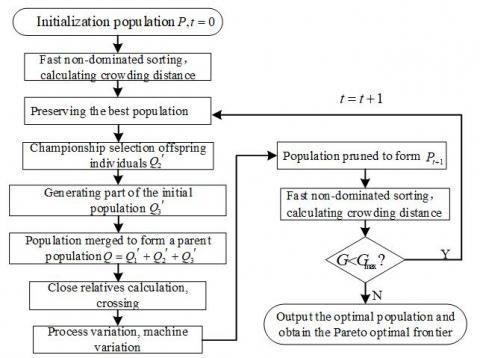
The non-dominated sorting genetic algorithm (NSGA) was proposed by Srinivas and Deb in 1994, and Deb then improved it, forming a NSGA-II algorithm [26]. In view of the characteristics of the flexible job shop, this paper adopts the interference coping strategy, and uses close relatives cross and variation to enhance the local search capability. In the iterative process, the elite strategy is used to accelerate the population convergence, and the new species group is introduced to improve the population diversity. The algorithm flow is shown in Figure 2.
Figure 2. NSGA-II algorithm flow based on crossover and mutation of close relatives
4.1 Scheduling problem coding
Since FJSP needs to solve such two problems as machine selection and process scheduling [27], the two-hierarchy encoding method [28] are used for process coding and machine coding. The FJSP is coded in a real number way, and the encoding way is like that in the literature [29]. For example, in the $3 \times 3$ fully flexible job shop scheduling problem (Total FJSP, T-FJSP), the chromosome gene is assumed to be $12323331122 : 2313311222$. The process gene is 1 2 3 2 3 3 1 1 2 2 and the machine gene is 2 3 1 3 3 1 1 2 2 2.
4.2 Interference coping strategy
When handling the interference, the earliest start time of each piece of work and machine needs to be reset. At the fault moment, the final completion time of each workpiece and each machine is also the earliest starting time of each workpiece and each machine. At this time, the completed process needs to be completed and the number of work-pieces in the population gene needs to be changed and the work-piece needs to be reordered.
4.3 Elite strategy and population diversity
The elitist strategy is adopted to preserve the individuals whose non-dominated sorting rank (Rank) is 1 and the crowding distance is not equal to 0 in the evolutionary process of each generation, and the best individual of the population is preserved in the manner of championship. In order to increase the population diversity, new populations are introduced in the evolution of each generation to improve the results of cross and mutation, and improve the searching ability of the population. Finally, the best-preserved individual and the newly generated population are taken as the parent together.
4.4 Crossover and mutation
(1) A cross method based on close relatives index
The NSGA-II algorithm is easy to lose the diversity of the population and falls into the local optimal, and the diversity of the population can be increased by intercrossing the progeny chromosomes. A larger cross probability is used for individuals with close blood relationships, and the cross probability is controlled between $p_{\text { cmin }}$ and $p_{\operatorname{cmax}}$ . Select two chromosomes randomly from the progeny population, and then calculate their relative index. The maximum close relatives index and the close relatives index of the last group of individuals are preserved and the cross probability is calculated, which is as shown in Eq. (19).
$p_{c}=p_{c \min }+\frac{\text {close}}{\text { max close }} \times\left(p_{\text {cmax}}-p_{\text {cmin}}\right)$ (19)
In this paper, the POX cross mode of literature [29] is adopted to inherit the excellent features of the parent generation [29], and the process and machine are adjusted accordingly during the cross time.
(2) Variation method based on close relatives index
The mutation probability affects the population’s local search ability. This paper confirms the population’s mutation probability using the maximum close relative index max close and the close relative index close of the last group of individuals which have been figured out using the above steps. The mutation probability is controlled between $p_{m m i n}$ and $p_{\operatorname{mmax}}$, which is as shown in Eq. (20).
$p_{m}=p_{m m i n}+\frac{\text {close}}{\max \text {close}} \times\left(p_{m \max }-p_{m \min }\right)$ (20)
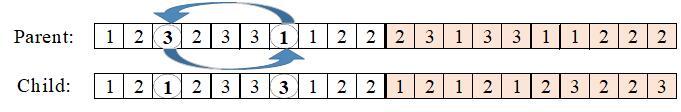
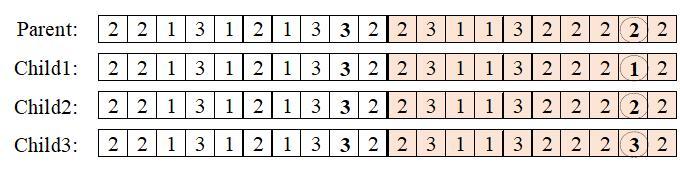
There are two approaches to genetic variation: First, a chromosome is randomly selected, and the process genes of the chromosome are exchanged. After the mutation, the machine gene violates the scheduling rule, so the second level machine gene is regenerated (see Figure 3). Second, once again, the gene is randomly selected, and a process is randomly selected for this gene. A good individual is selected in all available machines of the process (see Figure 4), and the inferior individuals will be deleted in the subsequent population pruning.
Figure 3. First step variation
Figure 4. Second step variation
4.5 Selection operation
NSGA-II algorithm uses fast non-dominated ranking and crowding distance to separate individual levels, and uses congestion comparison operator to ensure that the algorithm can converge to a uniform Pareto surface. In this paper, the fast non-dominated ranking method and congestion degree calculation method in literature [29] is adopted. The crowding degree comparison operator can maintain the diversity of population and maintain the stability of population size.
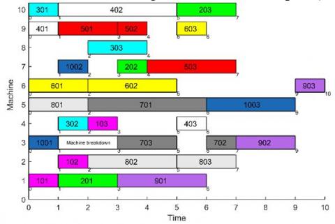
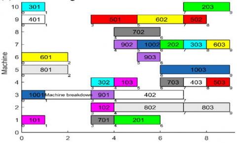
Figure 5. Initial Scheduling Scheme
Since there is no standard example for FJSP interference management, this paper takes 10×10 FJSP scheduling in literature [30] as an example. There are 10 workpieces and 10 machines, and the work process number for each workpiece is not necessarily equal. Each procedure can be implemented on multiple machines (the initial scheduling is as Figure 5). Process 201 represents the first process of workpiece 2, and 202 represents the second process of workpiece 2. After the initial execution of the original scheduling, machine 3 has a sudden failure at the timepoint of 1, and the fault processing requires 2 units of time. The occurrence of machine failure has a worsening effect on the processing of the subsequent process in the whole scheduling plan. The interference processing method is used to adjust the earliest available time of each workpiece, and the earliest available time of each machine is adjusted according to the interference management model. The risk attitude coefficient $\beta$ and the loss aversion coefficient λ of customers, manufacturers and workers used the typical values in literature [31], respectively. The algorithm is programmed on Matlab2015a, and the computer environment is the win10 system PC of Intel Core (TM) i5-2450 CPU2.50GHz with a Memory of 4GB. The size of the population is 100, and the maximum crossover probability of the evolutionary algebra 100 is 1. The minimum crossover probability is 0.3, the maximum mutation probability is 0.5, the minimum mutation probability is 0.01, and the mating pool size is 20.
5.1 Experimental result
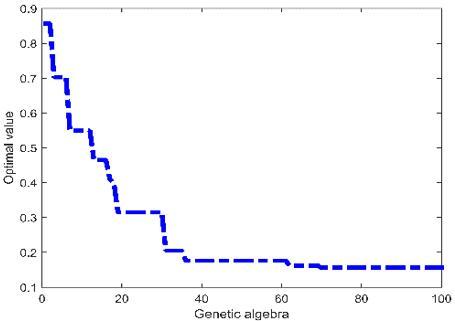
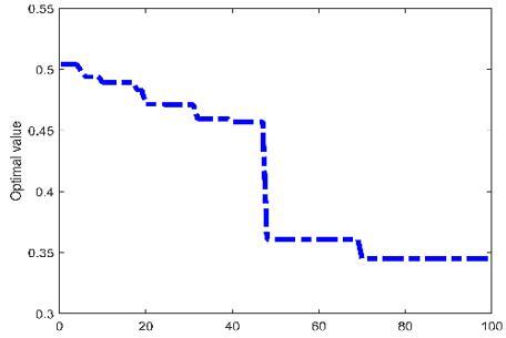
In the process of evolution, the target value is constantly optimized. Figure 6 is the optimization of the dissatisfaction target value of workers, manufacturer and workshop workers. The table 1 is optimal solution to the final generation of Pareto.
(a)The evolutionary process of the optimal value of the customer’s dissatisfaction
(b)The evolutionary process of the optimal value of the manufacturer’s dissatisfaction
(c)The evolutionary process of the optimal value of the workers’ dissatisfaction in the workshop
Figure 6. The evolutionary process of the best value of each objective function
Table 1. The optimal solution set to the final generation of Pareto
|
No. |
$f_{1}$ |
$f_{2}$ |
$f_{3}$ |
No. |
$f_{1}$ |
$f_{2}$ |
$f_{3}$ |
No. |
$f_{1}$ |
$f_{2}$ |
$f_{3}$ |
|
1 |
0.156 |
0.345 |
0.703 |
15 |
0.232 |
0.344 |
0.856 |
29 |
0.257 |
0.444 |
0.546 |
|
2 |
0.155 |
0.344 |
0.856 |
16 |
0.200 |
0.406 |
0.546 |
30 |
0.252 |
0.444 |
0.703 |
|
3 |
0.184 |
0.399 |
0.703 |
17 |
0.231 |
0.344 |
0.856 |
31 |
0.279 |
0.465 |
0.703 |
|
4 |
0.231 |
0.325 |
0.703 |
18 |
0.214 |
0.399 |
0.703 |
32 |
0.263 |
0.444 |
0.703 |
|
5 |
0.133 |
0.424 |
0.856 |
19 |
0.155 |
0.390 |
1.000 |
33 |
0.265 |
0.444 |
0.703 |
|
6 |
0.203 |
0.325 |
0.703 |
20 |
0.215 |
0.325 |
0.856 |
34 |
0.256 |
0.441 |
0.703 |
|
7 |
0.155 |
0.348 |
0.703 |
21 |
0.231 |
0.424 |
0.703 |
35 |
0.215 |
0.406 |
0.703 |
|
8 |
0.260 |
0.325 |
0.703 |
22 |
0.256 |
0.441 |
0.703 |
36 |
0.285 |
0.465 |
0.546 |
|
9 |
0.265 |
0.465 |
0.703 |
23 |
0.272 |
0.458 |
0.703 |
37 |
0.285 |
0.354 |
0.546 |
|
10 |
0.186 |
0.382 |
0.703 |
24 |
0.251 |
0.435 |
0.703 |
38 |
0.263 |
0.459 |
0.703 |
|
11 |
0.215 |
0.406 |
0.703 |
25 |
0.155 |
0.412 |
0.856 |
39 |
0.286 |
0.473 |
0.703 |
|
12 |
0.290 |
0.477 |
0.703 |
26 |
0.246 |
0.546 |
0.546 |
40 |
0.155 |
0.399 |
0.856 |
|
13 |
0.208 |
0.399 |
0.546 |
27 |
0.300 |
0.688 |
0.546 |
|
|
|
|
|
14 |
0.252 |
0.344 |
0.856 |
28 |
0.315 |
0.511 |
0.546 |
|
|
|
|
The algorithm finally gets the optimal solution set. According to the actual situation in production, the weight [19] of each target can be determined by AHP (analytic hierarchy process). This paper assumes that the target weights ω of $f_{1}$, $f_{2}$ and $f_{3}$ are 0.4, 0.4, and 0.2 respectively. Because the target value dimension has been unified, the comprehensive dissatisfaction $V_{i}$ is calculated directly as follow Eq. (21).
$V_{i}=\omega_{1} f_{1}+\omega_{2} f_{2}+\omega_{3} f_{3}$ (21)
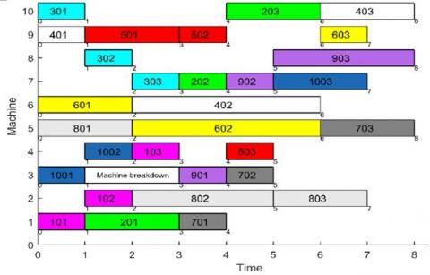
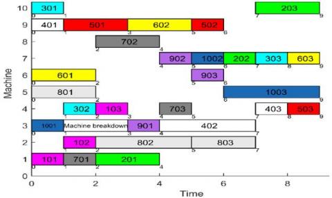
According to the results of the calculation of $V_{i}$, the optimal solution is finally obtained. The Gantt diagram is shown in Figure 7 (a) below. The results are compared with the results of rescheduling (Figure 7 (b)), right shift scheduling [6, 10] (Figure 7 (c)), and AOR rescheduling (Figure 7(d)). Table 2 is the comparison of the work completion time of the different scheduling methods (the italic and overstriking value is a tardiness piece). Table 3 is a contrast of dissatisfaction for different scheduling methods.
(a) Optimal scheduling scheme for interference management
(b) Rescheduling scheme
(c) Complete right shift scheduling scheme
(d) AOR rescheduling scheme
Figure 7. Comparison of scheduling schemes
Table 2. Comparison of work-pieces completion time under different scheduling methods
|
Workpieces |
Initial scheduling |
Interference management |
Rescheduling |
Fully right shift scheduling |
AOR rescheduling |
|
Job 1 |
3 |
3 |
3 |
5 |
3 |
|
Job 2 |
7 |
7 |
6 |
9 |
9 |
|
Job 3 |
6 |
4 |
3 |
8 |
8 |
|
Job 4 |
6 |
6 |
8 |
8 |
8 |
|
Job 5 |
7 |
7 |
5 |
9 |
9 |
|
Job 6 |
7 |
6 |
7 |
9 |
9 |
|
Job 7 |
5 |
5 |
8 |
7 |
5 |
|
Job 8 |
7 |
7 |
7 |
9 |
7 |
|
Job 9 |
4 |
10 |
8 |
6 |
6 |
|
Job 10 |
7 |
9 |
7 |
9 |
9 |
|
Makespan |
7 |
9 |
8 |
9 |
9 |
Table 3. Comparison of the results of different scheduling methods
|
Category |
Customer |
Manufacturer |
Worker |
Comprehensive dissatisfaction |
|
Fully right shift |
1 |
1 |
0 |
2 |
|
AOR rescheduling |
0.7 |
1 |
0 |
1.7 |
|
Rescheduling |
0.3 |
0.6 |
0.55 |
1.45 |
|
Interference Management |
0.2 |
0.38 |
0.7 |
1.28 |
5.2 Result analysis
For the scheduling results of rescheduling, fully right shift scheduling and AOR rescheduling, interference management scheduling can effectively reduce the comprehensive dissatisfaction of interference events to the whole manufacturing system. The reduction of disturbance to the manufacturing system by the disturbance management is mainly reflected in two aspects: the decrease of the number of the tardiness workpieces and the decrease of the total tardiness time.
(1) The number of the tardy work-pieces is reduced, so the customer’s dissatisfaction is reduced. As shown in Figure 7 (a), since the interference management method takes into account the interest demand of customers, there are only two delayed workpieces (workpiece 9 and workpiece 10) and parts of workpieces (workpieces 3) are completed ahead of schedule, which greatly reduces customer’s dissatisfaction. As in Figure 7 (b), rescheduling can minimize makespan, thus reducing the dissatisfaction of customers, manufacturers and workshop labors to a certain extent. But 3 work-pieces are delayed, and the overall dissatisfaction is high. As shown in Figure 7 (c), for the complete right shift scheduling, 10 workpieces are all delayed. The dissatisfaction of the customers and the manufacturers is the highest, which results in a greater degree of comprehensive dissatisfaction, while the dissatisfaction of the workers is the smallest. As in Figure 7 (d), AOR rescheduling has not delayed the completion time of partial workpieces because it pruned the unaffected process. There are 7 work-piece tardiness, and the manufacturers have the greatest degree of dissatisfaction, the customers’ dissatisfaction is reduced, and the workers’ dissatisfaction is the lowest.
(2) The total tardiness time is reduced, and the manufacturer’s dissatisfaction is reduced. The manufacturer’s benefit is determined by the total tardiness of the work piece, and the interference management takes into account the manufacturer’s requirements for different work periods. As a result, the total tardiness time is 8, and the total tardiness time of rescheduling, fully right shift scheduling and AOR rescheduling are 9, 20 and 14 respectively (Table 2).
In this paper, interference scheduling is based on the overall interests of the manufacturing system, and at the expense of the smaller interests of the laboring workers in the workshop, it achieves a significant decrease in the dissatisfaction of the customers and manufacturers, and balances the interests of the parties to the greatest extent, which is conducive to reducing the disturbance of the production system and improving the agility of the supply chain.
In this paper, aiming at the machine fault interference events in flexible job shop scheduling process, in order to reduce the gap between the scheduling theory and the actual scheduling effect, the behavioral subject’s perception in behavioral science and traditional operations research are combined, and an interference response method is proposed. The NSGA-II algorithm is improved to seek solutions efficiently. The work of this article is as follows:
(1) A method for measuring the disturbance of different behavior subjects in the workshop production system is proposed. By using the unascertained theory and prospect theory and combining the characteristics of different behavioral subjects in the event of disturbance, the unascertained measurement function of the behavior subject is established to quantify the dissatisfaction of different subjects. At the same time, the dissatisfaction of different behavior subjects is controlled within 0~1, and the disturbance can be compared more intuitively and accurately. The use of interference theory to solve practical problems can reduce the gap between production scheduling theory and production practice.
(2) A single machine fault interference management model in the process of production scheduling in flexible workshops is established. Aiming at the sudden failure interference of machine in the more complex FJSP, a disturbance management model considering the dissatisfaction of customers, manufacturers and workshop workers is established. In order to minimize the benefit loss of the whole manufacturing system, the Pareto optimal solution set is obtained to improve the ability to deal with the job shop scheduling interference. In the actual production, AHP and fuzzy comprehensive evaluation can be used to get different objective weights, and find the optimal scheduling from Pareto solution set, which is conducive to further improving the shop scheduling decision theory.
(3) The NSGA-II algorithm of crossover and mutation of close relatives is proposed to meet the need of real-time solution for production scheduling interference. According to the characteristics of FJSP, two layers of gene encoding, close relatives crossover, close relatives variation, integrating into new species and elite strategy are used to improve the NSGA-II algorithm. It is proved by an example that the algorithm can effectively solve the multi-objective optimization problem of FJSP. The algorithm is universally suitable for the production scheduling problem, which is beneficial to fast solving similar multi-objective optimization problems and obtaining the Pareto optimal solution set.
In this study, only some subjects and single interference events are considered, and the research on more subjects and interference events will be the focus of further research.
This research was supported by the key scientific research project of Henan Higher Education Institution (No.18B520023).
[1] Gao, L., Zhang, G.H., Wang, X.J. (2012). Flexible job shop scheduling algorithm and its application. Huazhong University of Science and Technology Press, Wuhan.
[2] Liu, Q., Zhang, Y.C., Rao, Q.Y., Shao, X.Y. (2009). Flexible job-shop scheduling problem with improved genetic algorithm. Industrial Engineering and Management, 14(2): 59-66. https://doi.org/10.3969/j.issn.1007-5429.2009.02.011
[3] Dobrin, C., Bondrea, I., Pîrvu, B.C. (2015). Modelling and simulation of collaborative processes in manufacturing. Academic Journal of Manufacturing Engineering, 3(13): 18-25.
[4] Kovács, G. (2017). Application of lean methods for improvement of manufacturing processes. Academic Journal of Manufacturing Engineering, 15(2): 31-36.
[5] Kuric, I., Císar, M. (2015). Machine tool errors and its simulation on experimental device. Academic Journal of Manufacturing Engineering, 13(4): 17-21.
[6] Liu, L., Zhou, H. (2013). Open shop rescheduling under singular machine disruption. Computer Integrated Manufacturing Systems, 10(10): 2467-2480. https://doi.org/10.13196/j.cims.2013.10.LIULe.20131012
[7] Zhang, J.W., Liu, G.T. (2015). Critical chain project scheduling problem with the robust objective. Journal of Systems Engineering, 30(1): 118-124. https://doi.org/10.13383/j.cnki.jse.2015.01.015
[8] Zhang, X.C., Zhou, H. (2012), A robust sing machine scheduling algorithm with rush orders. Industrial Engineering Journal, 15(5): 118-124. https://doi.org/10.3969/j.issn.1007-7375.2012.05.020
[9] Li, R.K., Shyu, Y.T., Adiga, S.(1993). A heuristic rescheduling algorithm for computer-based production scheduling systems. The International Journal of Production Research, 31(8): 1815-1826. https://doi.org/10.1080/00207549308956824
[10] Abumaizar, R.J., Svestka, J.A. (1997). Rescheduling job shops under random disruptions. International Journal of Production Research, 35(7): 2065-2082. https://doi.org/10.1080/002075497195074
[11] Mason, S.J., Jin, S., Wessels, C.M. (2004). Rescheduling strategies for minimizing total weighted tardiness in complex job shops. International Journal of Production Research, 42(3): 613-628. https://doi.org/10.1081/00207540310001614132
[12] Ding, Q.L., Jiang, Y. (2016), A model of disruption management based on behavioral operation research in production scheduling. Systems Engineering- Theory & Practice, 36(3): 664-673. https://doi.org/10.12011/1000-6788(2016)03-0664-10
[13] Jiang, Y., Sun, L. (2013), Model of disruption management with actors in sing machine scheduling. Journal of Mechanical Engineering, 49(14): 191-198. https://doi.org/10.3901/JME.2013.14.191
[14] Akturk, M.S. (2009). Predictive/reactive scheduling with controllable processing times and earliness-tardiness penalties. Iie Transactions, 41(12): 1080-1095. https://doi.org/10.1080/07408170902905995
[15] Louis, S.J., Xu, Z. (1996). Genetic algorithms for open shop scheduling and re-scheduling. ISCA 11th Intl. Conf. on Computers and their Applications, pp. 99-102.
[16] Wang, J.J., Liu, Y.J., Liu, F. (2015), Disruption management considering real-word behavioral participators in permutation flow shop. Systems Engineering-Theory & Practice, 35(12): 3092-3106. https://doi.org/10.12011/1000-6788(2015)12-3092
[17] Wang, D.J., Liu, F., Wang, Y.Z. (2016), Disruption management for new jobs arrivals with deteriorating effect and controllable processing times. Journal of Systems & Management, 25(05): 895-906.
[18] Chen, G., Gao, J., Sun, L.Y. (2007). A hybrid of genetic algorithm and bottleneck shifting for flexible job shop scheduling problems. Systems Engineering, 25(9): 91-97. https://doi.org/10.3969/j.issn.1001-4098.2007.09.016
[19] Chen, H.H., Jiang, Z.Q., Zuo, L., Zhang, Y.R. (2015). Multi-objective flexible job-shop scheduling problem based on nsga-II with close relative variation. Transactions of the Chinese Society for Agricultural Machinery, 46(4): 344-350. https://doi.org/10.6041/j.issn.1000-1298.2015.04.051
[20] Wu, X.L., Sun, S.D., Yu, J.J., Zhang, H.F. (2006). Research on multi-objective optimization for flexible job shop scheduling. Computer Integrated Manufacturing Systems, 12(5): 731-736. https://doi.org/10.3969/j.issn.1006-5911.2006.05.016
[21] Wei, W., Tan, J.R., Feng, Y.X. (2009). Multi-objective optimization method research on flexible job shop scheduling problem. Computer Integrated Manufacturing Systems, 18(8): 1592-1598. https://doi.org/10.13196/j.cims.2009.08.138.weiw.024
[22] Liu, Z.Y., Zha, Y., (2009), Behavioral operations management: An emerging research field. Journal of Management Science in China, 12(4): 64-74. https://doi.org/10.3321/j.issn:1007-9807.2009.04.007
[23] Piancastelli, L., Frizziero, L., Marcoppido, S., Pezzuti, E. (2011). Fuzzy control system for recovering direction after spinning. International Journal of Heat & Technology, 2(29): 87-94.
[24] D'Orazio, MC., Cianfrini, C., Corcione, M. (2000). An air-conditioning system based on the reverse Joule-Brayton cycle. International Journal of Heat & Technology, 18(2): 91-99.
[25] Liu, K.D., Cao, Q.K., Pang, Y.J. (2004), A method of fault diagnosis based on unascertained set. Acta Automatica Sinica, 30(5): 182-197.
[26] Deb, K., Pratap, A., Agarwal, S. (2002), A fast and elitist multiobjective genetic algorithm: NSGA-II. IEEE Transactions on Evolutionary Computation, 2(6): 182-197. https://doi.org/10.1109/4235.996017
[27] Wang, Y., Feng, Y.X., Tan, J.R., Li, Z.K. (2011). Optimization method of flexible job-shop scheduling based on multiobjective particle swarm optimization algorithm. Transactions of the Chinese Society for Agricultural Machinery, 42(2): 190-196. https://doi.org/10.3969/j.issn.1000-1298.2011.02.039
[28] Davis, L. (1985). Job shop scheduling with genetic algorithms. International Conference on Genetic Algorithms, L. Erlbaum Associates Inc, pp. 136-140.
[29] Zhang, C.Y., Rao, Y.Q., Liu, X.J. (2004). An improved genetic algorithm for the job shop scheduling problem. China Mechanical Engineering, 15(23): 83-87. https://doi.org/10.3321/j.issn:1004-132X.2004.23.020
[30] Xia, W.J., Wu, Z.M. (2005). An effective hybrid optimization approach for multi-objective flexible job-shop scheduling problems. Computers & Industrial Engineering, 48(2): 409-425. https://doi.org/10.1016/j.cie.2005.01.018
[31] Tversky, A., Kahneman, D. (1992). Advances in prospect theory: Cumulative representation of uncertainty. Journal of Risk and uncertainty, 5(4): 297-323. https://doi.org/10.1007/BF00122574