Approach to Reduce Throughput Time in Grinding of Gundrills

Gundrills are the straight fluted drill which allows cutting fluids (either compressed or suitable liquid) to be injected through drill’s hollow body to the cutting face. They are used for a deep drilling- a depth to diameter ratio of 300:1 is possible. A standard gundrill has a single effective cutting edge. Guide pads burnish the hole while drilling, allowing the hole to maintain straightness. The result of this burnishing activity is a very round hole with a precision diameter. Gundrill was initially developed for drilling gun barrels.

The gundrill is fabricated with a drill head section with carbide cutting blade. The head section is brazed to a heat treated tube (flute) section then fitted and brazed to hardened ground steel driver. The driver or shank, the single flute gundrill is provided with a driver for holding the tool in the machine spindle. A design methodology to sharpen the gundrill was developed by [1]. There are several types of carbide tip based on their coolant holes and guide pads. Tungsten carbide is one of the material used and their grinding method was discussed in the study carried out by [2]. The force system and performance of the welding carbide gun drill to cut AISI 1045 steel was discussed by [3]. Gun drilling in Inconel 718 for considering various parameters was discussed by [4]. Influence of preparation of surfaces on the tool life of the twist drills was studied by [5].

A cycle time of a job is the time required for the job to go through the factory. Reducing the cycle time is very important for the following factors. 1. Large cycle time means it is difficult to convert the opportunity cost into profits in the short term. 2. Results in accumulation of jobs resulting in bottleneck [6]. Throughput time is the amount of time required for a product to pass through a manufacturing process, thereby being converted from raw materials into finished goods. It covers the entire time from when it first enters manufacturing until it exits manufacturing which includes processing time, inspection time, move time and queue time. An algorithm to predict the throughput time was proposed by [7]. Calculating the throughput time of a production run is a complicated task [8-9]. A note on understanding the cycle time by [10] clearly showed the difference between cycle time, process time and throughput time. Process time is the period during which work is performed on job itself [11]. Manufacturing throughput time could be daunting task due to many factors that influence it and their complex interactions. Some guidelines to reduce throughput time are presented earlier like production and transfer batch size reductions offer the largest potential for MTTP (Manufacturing throughput time per part). If the plant has a job shop/ functional layout in place, significant reductions in batch size may require conversion to manufacturing cells which reduce move time, processing time, process variability and arrival variability further reducing MTTP [12]. Cellular manufacturing system is another method that helps in reducing throughput time [13]. An approach to reduce throughput time during the product design has been proposed by [14]. Design for production determines how new product design affects the performance which includes design guidelines, capacity analysis, and estimating throughput time [15].

This paper presents a study on the various grinding operations and identifies bottlenecks during gundrill production. Simulation is done in ARENA by Rockwell Automation Inc. for the manual process as well as for the automation required for the required for reduction in cycle time. Non-parametric tesats are conducted for validating the ARENA model.

The above problem is observed in manufacturing of gundrills in Kennametal India Ltd., due to high cycle times taken in the grinding processes couldn’t reach the targets in the specified period of time and the remaining components are piled up for the next installment. Table 1 show the timings noted for gundrills of diameter 8mm and 11.15 mm.

Table 1. Processing time for operations

The cycle timings of grinding operations which is creating bottleneck are shown in Table 2. The setup time is considered only for initial setup, for analysis purpose only process time is considered which includes the stage inspection. Here the grinding of gundrill follows the same sequences for all different diameter gundrill. The main aim is to reduce the throughput time which is carried out in analysis part.

Table 2. Processing time for grinding operations

Sl No	Operation	Dia=8.0 mm, Length=291 mm		Dia=11.5 mm, Length=901 mm
		Set up (min)	Process (min)	Set up (min)	Process (min)
1	OD roughing	0.83	13.3	1	14.32
2	OD finishing	0.66	10.53	1	13.17
3	Top rake roughing	0.5	7.16	1	6.22
4	Top rake finishing	0.5	6.25	0.83	5.63
5	Pad generation	0.66	13.71	1	14.50
6	Face geometry	0.83	16.78	1	17.13
Manual grinding		3.98	67.73	5.83	70.97
CNC grinding		2	50	4	40
Total time (min)		71.71		76.80

The reduction of cycle time for these operations is carried out in ARENA simulation software by Rockwell Automation Inc., for analysis purpose the area of interest will be the grinding operation which is shown in the Table 2. For simulation, gundrill having 8mm diameter is taken. The reason is if run-out can be maintained in smaller diameter gundrill then it is easy to maintain all machining activities for higher diameter gundrill. For 8mm diameter cycle timings are taken for a batch size of 25 numbers for grinding operations. ARENA provides built-in data analysis tool whose main objective is to fit distributions to a given sample. The distributions are analyzed for every grinding operation separately in the input analyzer tool. For OD roughing the histogram along with the distribution followed is shown in Figure 3.

3.png

Figure 3. Distribution for OD roughing

The distribution followed here is triangular. The data can fit in all other distribution as well. But analyzer follows the best possible by least square error value. Expressions are generated along with the distributions which will be used to define the process in particular operation. Table 3 shows the distributions, expressions, and least square value which will be used while creating the simulation model.

Table 3. Distribution summary

Operations	Distribution followed	Equation used	Error
OD roughing	Triangular	TRIA(12.8,13.2,13.6)	0.00738
OD finishing	Triangular	TRIA(10.2,10.6,10.8)	0.01555
Flute roughing	Weibull	5.31+WEIB(0.81,5.14)	0.04621
Flute finishing	Triangular	TRIA(5.73,6.17,6.36)	0.01021
Face generation	Beta	16.6+0.44xBETA(1.97,1.61)	0.029915
Pad generation	Beta	13.5+0.42x BETA(1.5,1.55)	0.011172

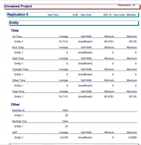
After distribution analysis is completed a model is created in ARENA. The model is started with a basic process called create which is labeled as parts to be grinded followed by the individual process. The process is defined based on the delay type and expressions which are generated in input analyzer shown in Table 3. Allocation is defined as value added time because the non-value added time in the conventional method is very few seconds and it is negligible. Similarly every other operation is defined in the same way along with the decision block which is stage inspections which may be either roughness or diameter check. If it satisfies the condition it is carried moved to further processes. When the above model is simulated for batch size 25 and for ‘n’ replications the result of total average timing of all operations is shown in Figure 4. Since only value added time is considered, non-value added time, wait time, transfer times are zero for the reason that all other times are negligible during the process. To find the average cycle timings of each individual process model is created to each single process similarly using the expressions and procedures and simulation is carried out and results are tabulated in Table 4.

4.png

Figure 4. Simulation result for conventional model

Table 4. Average cycle timings for grinding operations by ARENA

Sl No	Operations	Avg. Time (mins)
1	OD roughing	14.66
2	OD finishing	11.61
3	Flute roughing	6.71
4	Flute finishing	6.76
5	Face generation	18.67
6	Pad generation	15.37
Total		73.78

 

3.1 Validating ARENA model

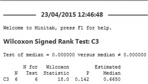
To find whether the ARENA model resembles the conventional method, a non-parametric test is done by checking null hypothesis and checking p-value. Usually non- parametric test is done when the data is assumed to be not following the normal distribution. For non-parametric test Wilcoxon signed rank test is carried out for two samples. It is a non-parametric statistical hypothesis test used to compare two related samples, matched samples, or repeated measurements when the population cannot be assumed to be normally distributed. For the test average timings from individual operations from shop floor and average individual results of simulation model is taken.  Null hypothesis test is conducted with 5 % significance level and p-value is calculated. The Wilcoxon signed rank test for two samples is carried out in mini- tab and results are shown in Figure 5.

5.png

Figure 5. Wilcoxon signed rank test for null hypothesis

The p-value is greater than the significance value i.e. p>0.05 which shows the weak evidence against the null hypothesis, so fails to reject the null hypothesis. This proves the median of ARENA timings and median of manual reading are equal. This further justifies the resemblance between ARENA model and manual readings from shop floor.

3.2 ARENA for CNC

For the special purpose CNC machine since there is no data for finding distributions and run a model in ARENA alternate way of assuming distributions is done. When distributions are not known triangular distributions is commonly used in these circumstances. It estimates for the minimum, maximum and most likely values available. The triangular distributions are easier to use and explain than other distributions and may be used in this situation [6]. The minimum, maximum and most likely values are taken from the timings which is taken from floor is used to define the process for CNC and another model is created similarly to the manual ARENA model as shown in Figure 6.

Here the procedure for model creation goes same except while defining the process instead of expression every process is assumed to be following the triangular distribution and minimum, maximum and most likely value is given as input. Since it is a CNC grinding machine no stage inspections are involved as in manual method, when simulated results are generated as shown in Figure 7. The total cycle timing which is given by ARENA is following the same condition as in manual process i.e. feed rate, depth of cut and all other grinding parameters. The cut-off timings for all grinding operations are shown in Table 5.

For the same ARENA model in Figure 6, for all cycle timings having maximum, minimum and the mode (most likely value) the values are reduced a value of 75 % for all operation and model is simulated the average final value is shown in Figure 8. The cut-off timings for all individual operations are shown in Table 6. Here the total cycle timing is reduced to 16.44 mins. This reduced cycle times means the main machining parameters like feed-rate and depth of cut considered here for conventional as well as for proposed CNC when increased by certain percentages the cycle timings can be reduced and the target can be achieved.

Table 7 shows the comparison of the results obtained from manual, ARENA and CNC methods.

6.png

Figure 6. Simulation model for CNC

7.png

Figure 7. Simulation results for CNC model

8.png

Figure 8. Cycle timings for 75 % reduction

Table 5. Average cycle timings for CNC

Sl No	Operations	Avg. Time (mins)
1	OD roughing	13.22
2	OD finishing	10.5
3	Flute roughing	5.94
4	Flute finishing	6.05
5	Face generation	16.79
6	Pad generation	13.67
Total		66.17

 

Table 6. Cycle timings of individual operation for CNC 75 % reduction

Sl No	Operations	Avg. Time (mins)
1	OD roughing	3.29
2	OD finishing	2.6
3	Flute roughing	1.47
4	Flute finishing	1.5
5	Face generation	4.18
6	Pad generation	3.4
Total		16.44

 

Table 7. Comparison of results

Operations	Manual (mins)	Manual ARENA (mins)	ARENA for CNC (mins)	CNC 75 % (mins)
OD roughing	13.3	14.66	13.22	3.29
OD finishing	10.53	11.61	10.5	2.6
Flute roughing	7.16	6.71	5.94	1.47
Flute finishing	6.25	6.76	6.05	1.5
Face generation	16.78	18.67	16.79	4.18
Pad generation	13.71	15.37	13.67	3.4
Total	67.73	73.78	66.17	16.44