Pranati Mishra*![]() | Ranjan Kumar Dash
| Ranjan Kumar Dash![]() | Tanpriya Choudhury
| Tanpriya Choudhury![]() | Kitan Kotecha
| Kitan Kotecha
© 2024 The authors. This article is published by IIETA and is licensed under the CC BY 4.0 license (http://creativecommons.org/licenses/by/4.0/).
OPEN ACCESS
For reliable use of wireless sensor networks, energy, and delay optimization are equally crucial. Packets must therefore be routed via the path with the least amount of delay and energy consumption possible. For both clustering and non-clustering WSN scenarios, this problem remains an exploratory challenge. The optimization problem is presented here as a multi-objective problem in the clustering and non-clustering WSN contexts. A new energy model is presented for Wireless Sensor Networks (WSN) that has two more components: switching between transmission and reception modes and using the CSMA/CA protocol for packet transfer. This optimization problem is solved in two working environments: clustering and non-clustering, using a stochastic optimization technique particle swarm optimization (PSO) that uses particles to explore the search space. The proposed PSO-based approach increases WSN lifetime by 45% over ACO and twice as much as GA when compared to Genetic Algorithm (GA) and Ant Colony Optimization (ACO). The result additionally demonstrates the WSN's delay-tolerant routing in two operational scenarios. The proposed routing framework offers the potential for prolonging the lifetime of WSNs in many real-time applications, including area monitoring, healthcare monitoring, habitat monitoring, and industrial monitoring.
residual energy, particle swarm optimization, WSN lifetime, energy model, shortest path
Routing refers to the method of directing data transmission from its origin to its intended endpoint. In wireless sensor networks, the primary goal of routing techniques is to establish a pathway between source node to the base station. Length of such a path bears paramount importance when it is required to optimize energy consumption. A long path with more participating intermediate sensor nodes consumes more energy than a shorter path with fewer intermediate nodes. The reason is straightforward from the observation that a longer path requires more delay for establishing the whole connecting path in which each sensor node sends or acknowledges some control signals for the wireless link setup between them. Hence, the shorter path, or more precisely, a minimal path, is an appropriate choice for less energy consumption [1]. Energy consumption stands as the pivotal factor influencing the lifespan of sensor networks due to their reliance on battery power for most sensor nodes. Optimizing energy usage presents a formidable yet indispensable challenge in sensor networks, aiming to minimize energy consumption. The sensor nodes which are the core components of WSN have limited processing speed, storage capacity, and communication bandwidth [2]. Natural computing solutions have arisen because of traditional or conventional computing techniques failing to meet real-world challenges [3].
In the study by Srivastava et al. [1-3], several clustering approaches are over-represented, while the non-clustering environment is mostly overlooked. In many real-time applications, designing sensor node clustering is often impractical within WSNs. The clustering of sensor nodes is either ineffective or challenging to implement, particularly with the emergence of recent techniques such as the Internet of Things. In this scenario, energy optimization must be pursued within a non-clustering WSN environment. WSN can assemble data and sense packages and deliver them to the base station via intermediate nodes known as hubs in a non-clustering setting. As a result, in order to preserve energy, the number of nodes should be reduced to a minimum. To put it another way, the problem can be thought of as a multi-objective problem with the purpose of lowering energy consumption by taking the shortest path.
This paper's study aims to extend the lifespan of WSNs by introducing PSO-based routing frameworks for both clustering and non-clustering working models. The rest of the paper as: Section 2 elaborate the related work, Section 3 introduces the energy model and PSO-based algorithms utilized for optimizing the residual energy of WSN, and Section 4 presents the simulated results along with a discussion. Finally, Section 5 offers the paper's concluding remarks.
Patil et al. [4] proposed AADITHYA, a novel AEB-AODV (Available Energy Based AODV) and Ad-hoc On Demand Distance Vector routing protocols. Simulations show superior performance, but challenges include limited real-world validation and implementation complexity. Study by Singh et al. [5] identifies criteria for optimal energy use in sensor nodes. Results suggest extended battery life via genetic algorithm parameter selection, despite implementation challenges and scenario-dependent effectiveness. Guleria and Verma [6] developed a procedure grounded in Load-Balanced Cluster-Based Routing Protocol Utilizing ACO for optimal cluster head selection, outperforming others by considering residual energy in addition to the probability weight factor. Energy conservation achieved [7] by activating the radio only during broadcasting with a fault-tolerant MAC protocol and node scheduling. Enhanced efficiency, potential limitations in protocol complexity. Hu et al. [8] tackle unequal energy consumption in WSNs, addressing issues like uneven power usage and premature node death using two routing algorithms [9]: multipath and optimal routing. This paper by Li et al. [10], using ant colony principles for WSNs, optimizes energy consumption, enhancing load balance and stability. Prioritizing higher residual energy nodes extends network lifespan. The study of Arya et al. [11] compares Energy Aware Routing with and without ACO, finding ACO minimizes energy consumption as nodes increase, extending lifespan. The energy consumption in WSN was optimized with the Neuro-Fuzzy Inference System (ANFIS) in this work [12]. The research work by Cao and Zhang [13] refined the stable election procedure (SEP) for extending the lifetime of WSNs in a variety of environments. Authors of this research work [14] proposed a collaborative approach for multiple requests in service-oriented WSNs. The proposed technique boosted service sharing and lowered energy usage in a WSN network. The enhanced energy optimization routing protocol improves upon PARPEW (predictive and adaptive routing protocol utilizing energy welfare) model in the study by Wang et al. [15] by addressing its drawbacks. It introduces a refined head selection method based on residual energy, reducing intra-cluster communication energy. Bojan and Nikola [16] proposed a method for reducing consumption of energy during data packet transmission in WSN by employing a genetic algorithm. Different techniques have been discussed by Bouazzi et al. [17] for the improvement of life time as well as energy in wireless sensor networks. A sleep algorithm [18] for nodes of a random wireless sensor network was proposed to reduce energy consumption. The CMIMO (Cooperative Multi-Input Multi-Output) technology was studied for intra-cluster communication. An approach has been proposed by Al-Khayyat and Ibrahim [19] that used Ant Colony Optimization and K-means clustering to deliver optimal routing without requiring infrastructure or individual nodes. The protocolooptimizes energy [20] in WSN through dynamic selection of high residual energy nodes using energy regions. Bahadur and Lakshmanan [21] introduced a meta-heuristic GA-based algorithm by using different parameters like selection, crossover, fitness function, and mutation. It provides an optimized result in network coverage instead of random deployment. In the study by Roberts and Ramasamy [22], the study combined the Golden Eagle Optimization Algorithm with enhancements to the Grasshopper Optimization Algorithm to introduce an improved cluster-based routing protocol named GEIGOA. Gunigari and Chitra [23] introduced an Energy-Efficient and Reliable Routing Protocol using genetic algorithm (GA). The HPSO-ILEACH hybrid method [24] optimizes cluster head selection in WSNs, enhancing load balancing, power efficiency, and network stability. Most techniques discussed so far use a traditional energy model, such as the power model [25, 26], but in practice, energy consumption use is governed by rather than bound by the assumptions established in the power model.
This work adopts a different energy model for WSN. Further, the above-mentioned works presented clustering techniques to reduce energy consumption. The cluster head is picked at random or according to criteria such as least distance node, largest residual energy, and so on in these methods. On the other hand, distance-based clustering algorithms have been found to be more effective than other techniques. As a result, the challenge of energy consumption becomes a multi-objective problem, wherein energy conservation is achieved by selecting the best cluster head with both the shortest distance from the cluster center and the highest remaining energy.
The majority of the research works mentioned above are aimed at minimizing energy consumption in WSNs by proposing various energy-efficient clustering techniques. Depending on the situation, they frequently apply heuristic or meta-heuristic procedures to address single or many objective domains. Techniques like the Genetic Algorithm and its variations, as well as Particle Swarm Optimization, are examples of population-based methodologies. Although the Genetic algorithm typically fails to yield a global optimal solution, it is a popular choice among academics due to its simplicity and minimal number of required hyper parameters. When compared to Genetic Algorithms, Ant Colony Optimization requires significantly more hyper parameters to operate over the same issue area, but delivers a more competent optimal solution. While there are limited instances in the literature employing Particle Swarm Optimization (PSO), numerous research studies, including references [27, 28], acknowledge PSO as a fast and efficient approach. Furthermore, PSO necessitates fewer hyper parameters than ACO. Consequently, PSO can serve as a strategy to reduce consumption of energy in application of WSNs with lower computational demands. The aforementioned concerns motivate us to research multi-objective residual energy minimization and its solution using PSO.
1. The study's major purpose is to find a more appropriate energy model for WSNs.
2. The residual energy maximization problem is formulated in two alternative working environments: clustering and non-clustering.
3. The particle swarm optimization-based technique is used for two different contexts.
4. It also provides a thorough examination of the simulated results.
The WSN comprises 'n' sensor nodes deployed under certain assumptions, as outlined below:
(i) All selected nodes are assumed to remain stationary after deployment.
(ii) Two distinct types of nodes are: nodes for environmental sensing, sink or base stations positioned at the middle of the WSN.
(iii) Sensors are assigned unique identification (ID) numbers and have similar remaining energy levels.
(iv) Assume that all links between nodes are symmetric.
Within the WSN, an energy model is designed at the physical layer to calculate energy losses in every sensor node during the other sensor nodes communication.
3.1 Energy model of wireless sensor network
Let us consider that the WSN consists of $n$ numbers of randomly distributed nodes over an area of $\mathrm{A} \mathrm{m}^2$. Initially, each sensor node has the same amount of energy i.e. $E_I\left(N_i\right)$, where, $N_i$ is the $i_m^{\text {th }}$ sensor node. Sensor node incurs energy consumption for the following reasons:
The sensor node either sends its own packets or forwards the packets of other nodes. If size of each packet is $\varpi$ and the number of packets transmitted by each node is $P_T$, total energy consumed to send $P_T$ can be expressed as:
$E_T\left(N_i\right)=\varpi P_T$ (1)
Similarly, the energy consumption for receiving $P_R$ number of packets is written as:
$E_R\left(N_i\right)=\varpi P_R$ (2)
Considering the above-mentioned factors, the consumption of energy by every sensor node can be expressed as:
$E_C\left(N_i\right)=E_T\left(N_i\right)+E_R\left(N_i\right)+E_S\left(N_i\right)+E_{C S M A}\left(N_i\right)$ (3)
The rest energy of each sensor node at time (t) can be calculated as:
$E_R\left(N_i\right)=E_I\left(N_i\right)-E_C\left(N_i\right)$ (4)
The total residual energy ($E_{T R}$) of n number of sensor nodes can be calculated from Eq. (4) and is presented below:
$E_{T R}=\sum_{i=1}^n E_I\left(N_i\right)-\sum_{i=1}^n E_C\left(N_i\right)=n \times E_I\left(N_i\right)-\sum_{i=1}^n E_C\left(N_i\right)$ (5)
The transmitted packets by the sensor nodes must follow some specific paths to reach the base station. Such paths are represented by means of the nodes and the link connecting them. Mathematically, these paths can be expressed as a conjunction of the different wireless links i.e.
Path $=\Lambda_{i, j=1}$ todand $i \neq j\left(N_i, N_j\right)$ (6)
where, $N_d$ is the base station.
To optimize each sensor node’s energy, it is required to minimal the transmission paths i.e., it contains a smaller number of nodes than other paths. Thereby ensuring that a smaller number of nodes become the intermediate nodes during the transmission. Further, transmitting packets through minimal paths minimizes the network delay, which is a function of the following parameters:
3.2 Optimization of residual energy for non-clustering environment
In a non-clustering environment, each node sends its packets to its nearest neighbour for further transmission. Consequently, the probability of a neighbouring node serving as an intermediate node during packet transmission remains uniform across different neighbour nodes. Therefore, for reducing overall energy consumption is to choose the shortest paths between each sensor node and the base station. It can be represented as $|p a t h|_p$, where 'p' denotes the total number of paths and $\mid$ path $\mid$ indicates the length of the path.
Maximization of residual energy of WSN can be formulated mathematically, as
Maximize $E_{T R}$ (7)
Subject to constraints
$\min _{i=1,2, \ldots . . p} \mid$ path $\left.\right|_p$ (8)
$\sum_{i=1}^n \mathrm{E}_{\mathrm{C}}\left(N_i\right) \leq T_E$ (9)
$1 \leq i \leq n$ (10)
In the above-mentioned problem, the constraint (8) ensures a minimal path for transmission of packets within the source node and the destination. The total energy consumption by the WSN at any particular time (t) must have an upper bound $T_E$, which is represented by constraint (9). Once, the upper bound is achieved, no further maximization of total residual energy is possible. Constraint (10) is trivial in nature.
3.3 Optimization of residual energy for Clustering Environment
The clustering of sensor nodes provides many benefits including less overall energy consumption by WSN [28]. However, considering the energy consumption model, a sensor node can be a cluster node if the ratio of its energy consumption and its residual energy must be greater than some threshold value (T). Otherwise, the node gradually becomes dead node and this significantly reduces the overall performance of the WSN. Mathematically, it can be expressed as:
$\frac{E_C\left(N_i\right)}{E_r\left(N_i\right)}>T$ (11)
For each cluster $\left(C_k\right)$, the inter distance between the sensor node and the cluster head $(\mathrm{CH})$ can be expressed as $d\left(N_i, \mathrm{CH}\right)$, where, $N_i \in C_k$. The sum of these distances is:
$D\left(C_k\right)=\sum_{i=1}^{\left|C_k\right|} \mathrm{d}\left(N_i, C H\right)$ (12)
The average distance between the sensor node and the clustering head is calculated as:
$\operatorname{Avg}\left(C_k\right)=\frac{D\left(C_k\right)}{\left|C_k\right|}=\frac{1}{\left|C_k\right|} \times \sum_{i=1}^{\left|C_k\right|} \mathrm{d}\left(N_i, C H\right)$ (13)
If there are k numbers of clusters, the minimum average distance can be computed as:
$\min _{k=1,2, \ldots . k}\left\{\sum \forall N_i \in C_k \frac{d\left(N_i, C H_k\right)}{\left|C_k\right|}\right\}$ (14)
By using Eqs. (5), (11) and (14), the maximization problem can be formulated as:
Maximize $E_{T R}$ (15)
Subject to constraints
$\begin{gathered}\frac{E_C\left(N_i\right)}{E_r\left(N_i\right)}>T \\ \min _{k=1,2, \ldots k}\left\{\sum \forall N_i \in C_k \frac{d\left(N_i, C H_k\right)}{\left|C_k\right|}\right\}\end{gathered}$
Mapping of PSO to routing problem.
Particle swarm optimization technique consists of a predefined number of particles (np). Each particle (Pi) provides a solution to the optimization problems defined in (7) and (15). The particles have their own position (Xi,j) and velocity defined within the search space of dimension(D). The positional vector of each particle is defined as:
$P_i \cdot$ position $=\left\{X_{i, 1}, X_{i, 2}, X_{i, 3} \cdots X_{i, D}\right\}, 1 \leq i \leq n_p$ (16)
Similarly, the velocity of each particle can be represented by a D-dimensional vector
$P_i$. Velocity $=\left\{V_{i, 1}, V_{i, 2}, V_{i, 3} \cdots V_{i, D}\right\}, 1 \leq i \leq n_p$ (17)
The above-mentioned mapping of PSO for solving WSN routing problem can be explained by taking a two-dimensional search space. Thus, each particle has a location in this space with appropriate X and Y coordinate values. For example, P0(100,50) provides the location of particle P0 with 100 and 50 as its X and Y coordinate values. Similarly, the velocity of each particle can also be explained in two-dimensional space.
The fitness function is used to evaluate each particle to ensure the quality of the solution. The best solution obtained for each particle is called its PBesti while the best solution among the particles is termed as Gbest. The particle updates its position and velocity with respect to the Pbest value. This updating process continues till get the optimal result. The velocity and position of each particle is updated by the following equations:
$V_{i, j}^{t+1}=w \times V_{i, j}^t+r_1 \times c_1 \times\left(P B \operatorname{Best}\left(X_{i, j}^t\right)-X_{i, j}^t\right)+r_2 \times c_2 \times\left(\operatorname{GBest}\left(X_{i, j}^t\right)-X_{i, j}^t\right)$ (18)
$X_{i, j}^{t+1}=X_{i, j}^t+V_{i, j}^{t+1}$ (19)
where, $r_1, r_2$ are the random numbers between 0 and 1,
$w$ is weight parameter,
$c_1, c_2$ are the weight factors.
In this study, each particle symbolizes a path originating from a sensor node (or cluster head) to the base station. The quantity of particles $\left(n_p\right)$ corresponds to the number of sensor nodes, maintaining a one-to-one mapping relationship between sensor nodes and particles.
3.4 Proposed PSO based routing algorithm for non- clustering environment
The PSO-based routing algorithm in a non-clustering environment comprises the following three key steps:
The number of particles is equal to the number of sensor nodes. Each particle's position and velocity are initialized to values generated randomly from a uniform distribution. The dimensions of the particles are consistent and equal to the number of particles (np) in the population.
Thus,
$P_i$. position $=\operatorname{rand}\left[0, n_p\right]\{\sim$ Uniformdistribution $\}$
where, $1 \leq i \leq n_p$
Similarly, the velocity of each particle is initialized as:
$P_i . \text { velocity }=\operatorname{rand}\left[0, n_p\right]\{\sim \text { Uniformdistribution }\}$
Maximization of residual energy of WSN can be achieved by allowing the sending of packets through the minimal paths. Thus, the problem is multi objective in nature where residual energy is maximized while the length of the traversal path is minimized. It is intuitive to believe that a shorter path is associated with shorter delay as compared to a longer one.
By using Eqs. (7) and (8) the fitness function (F) can be written as
$F=\alpha\left(E_{T R}\right)+(1-\alpha)\left(\min _{i=1.2 \ldots \ldots p} \mid\right.$ path $\left.\left.\right|_p\right)$ (20)
where, $\alpha$ is control parameter to maximize the residual energy $\left(E_{T R}\right)$ while $(1-\alpha)$ minimizes the path length and hence the network delay. Normally, $\alpha$ lies between 0 and 1 i.e. $0<\alpha<1$.
The velocity and position of each particle is updated in every iteration by the Eqs. (18) and (19). The particles having the new position and velocity are evaluated by the fitness function defined in (20). Accordingly, the PBest$_i$, where $1 \leq i \leq n_p$ and GBest are calculated by using the Eq. (20). The updation rules for updating PBest$_i$ and GBest are presented below:
PBest $_i=\left\{F\left(P_i\right)\right.$ if $F\left(P_i\right)>$ PBest$_i$ PBest$_i$ otherwie (21)
GBest $=\left\{F\left(P_i\right)\right.$ if $F\left(P_i\right)>$ GBest$_i$ GBest otherwie (22)
Algorithm- PSO_Routing_NCE ($n_p$)
for each particle Pi, $\mathbf{1} \leq \boldsymbol{i} \leq \boldsymbol{n}_{\boldsymbol{p}}$
$\begin{aligned} & P_i \cdot \text { position }=\operatorname{rand}\left[0, n_p\right]\{\sim \text { Uniformdistribution }\} \\ & P_i \cdot \text { velocity }=\operatorname{rand}\left[0, n_p\right]\{\sim \text { Uniformdistribution }\}\end{aligned}$
endfor
for each particle Pi, $\mathbf{1} \leq \boldsymbol{i} \leq \boldsymbol{n}_{\boldsymbol{p}}$
Compute F(Pi) by using Eq. (20)
PBesti = F(Pi)
endfor
Find GBest$=\max _{1 \leq i \leq n_p}\left\{\right.$ PBest $\left.{ }_i\right\}$
while(!termination)
for I =1 to np
Update velocity and position of Pi by using equation(18) and (19)
Calculate F(PI)
if F(Pi) >PBesti then
PBesti=f(Pi)
endif
ifPBesti>GBest then
GBest= PBesti
endif
endfor
if Gbest<=0
break
end if
endwhile
Generate the route for each sensor node (Si), $1 \leq i \leq n$ by using GBest
Stop
Computational complexity and Convergence criteria of the algorithm PSO_Routing_NCE( )
The convergence criterion of the proposed algorithm is if Gbest<=0. The while loop stops its repetition onceGbest<=0. Let It be the number of times that while loop is repeated in its execution. The inner for loop is executed np times and hence the computational complexity of the proposed algorithm is found to be $O\left(I t \times n_p\right)$.
3.5 Proposed PSO based routing algorithm for clustering environment
Similar non-clustering environment, the PSO based energy efficient routing algorithm for clustering environment also consists of the following three major steps:
Most of the initialization process for a non-clustering environment remains the same as for the clustering environment. However, in the non-clustering scenario, the number of particles is now dictated by the count of cluster heads. This is due to all sensor nodes within a cluster being connected to their respective cluster head, necessitating packet transmission to traverse intermediate cluster heads en route to the base station.
The fitness function for clustering environment can be defined by using the Eqs. (14) and (15) as:
$F=\propto\left(E_{T R}\right)+(1-\propto)\left(\min _{k=1,2, \ldots \ldots . . k}\left\{\sum \forall N_i \in C_k \frac{d\left(N_i, C H_k\right)}{\left|C_k\right|}\right\}\right)$ (23)
where, α is control parameter to maximize the residual energy while (1-α) minimizes the distance between the node and the cluster head. The value of α lies between 0 and 1 i.e. $0<\alpha<1$.
The updation of the velocity and position for each particle are carried out as per the Eqs. (18), (19), (20) and (21).
Algorithm- PSO_Routing_CE ($n_p$)
for each particle Pi, $\mathbf{1} \leq \boldsymbol{i} \leq \boldsymbol{n}_{\boldsymbol{p}}$
$\begin{aligned} & P_i \cdot \text { position }=\operatorname{rand}\left[0, n_p\right]\{\sim \text { Uniformdistribution }\} \\ & P_i \cdot \text { velocity }=\operatorname{rand}\left[0, n_p\right]\{\sim \text { Uniformdistribution }\}\end{aligned}$
endfor
for each particle Pi, $1 \leq \boldsymbol{i} \leq \boldsymbol{n}_{\boldsymbol{p}}$
Compute F(Pi) by using Eq. (23)
PBesti = F(Pi)
endfor
Find GBest$=\max _{1 \leq i \leq n_p}\left\{\right.$ PBest $\left._i\right\}$
while(!termination)
for I =1 to np
Update velocity and position of Pi by using equation(18) and (19)
Calculate F(PI)
if F(Pi) >PBesti then
PBesti=f(Pi)
endif
ifPBesti>GBest then
GBest= PBesti
endif
endfor
if Gbest<=0
break
end if
endwhile
Generate the route for each cluster head (CHk), $1 \leq i \leq\left|C_k\right|$ by using GBest
stop
Computational complexity and Convergence criteria of the algorithm PSO_Routing_CE( )
The computational complexity and convergence criteria mentioned for algorithm PSO_Routing_NCE() are same forPSO_Routing_CE().
The simulation is performed by Python in Google Collab environment. This section is divided in to three parts:
4.1 Comparing the PSO-based approach with methods using GA and ACO
The proposed PSO based residual energy optimization method is compare against the genetic algorithm and ant colony optimization techniques. The different parameters of GA and PSO are selected [29] and accordingly, the parameters of GA and ACO are set for simulation purposes (Table 1).
Table 1. Parameters of GA, ACO and PSO
|
Genetic Algorithm |
Population size |
100 |
|
Cross over rate |
0.9 |
|
|
Mutation rate |
0.1 |
|
|
Ant Colony Optimization |
Number of ants |
100 |
|
Parameters controlling the relative importance of pheromone |
0.8 |
|
|
3, 3 |
||
|
The pheromone reward factor |
50,000 |
|
|
The pheromone penalty factor |
0.0015 |
|
|
Particle Swarm Optimization |
Swam size |
100 |
|
Weight factor |
2, 2 |
|
|
Weight parameter |
0.9 |
100 number of cluster nodes have been considered over a target region of 1000 m × 1000 m with a transmission range value 150 for each sensor nodes. The sensor nodes are randomly placed throughout the designated area. Three above mentioned methods are simulated to optimize the residual energy of WSN. The results obtained are showed in Figure 1 and Figure 2 respectively.
Figure 1. Residual energy maximization by proposed method, method based on GA and ACO
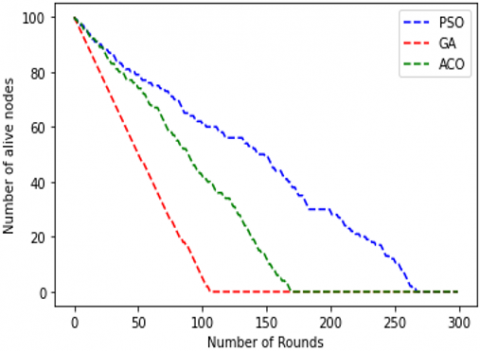
Figure 2. Life span maximization by proposed method and method based on GA
The residual energy of the sensor node becomes zero after roughly 70 iterations in the case of GA, but the residual energy of the node becomes zero after around 220 iterations in the case of ACO, as shown in Figure 1. The suggested PSO algorithm, on the other hand, can run for up to 260 iterations before the residual energy of node zero is reached.
The graphical representation (Figure 2) demonstrates that the proposed PSO-based technique consistently produces the best results. In comparison to the methods GA and ACO, the proposed strategy maximises life span. The alive nodes can survive for 260 iterations, which is significantly longer than the other two optimization strategies, ACO and GA
4.2 Residual energy maximization of WSN under non-clustering environment
(a)
(b)
Figure 3. Routing through minimal path (a) and through longest path (b)
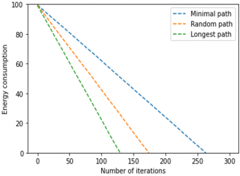
Figure 4. Residual energy maximization by proposed method considering three different paths
In order to analyze the impact of path length on routing among the sensor nodes as well as the base station, twenty number of sensor nodes are randomly distributed in a target area of 100x100 m2. The residual energy of WSN is maximized by using the algorithm for three distinct cases of path length (shown in Figure 3):
The simulated results obtained are shown in Figure 4 is quite apparent which in turns ensures the ability of new algorithm to maximize the residual energy of WSN under even hostile environment like choosing the longest path if required.
4.3 Residual energy maximization of WSN under clustering environment
(a)
(b)
Figure 5 Routing in clustering environment of WSN through minimum distance (a) and through maximum distance (b)
Figure 6. Residual energy maximization by proposed method considering three distances from cluster head
To carry out the simulation, 100 number of sensor nodes are randomly placed in 100 × 100 m2 target area. Five number of energy efficient clusters are created among these nodes by using method. Three different distances are taken as parameters to select the cluster node while rest parameters are same as mentioned in [29]. The PSO based algorithm is used to maximize the residual energy for each case (Figures 5 and 6).
The above result shows that the energy consumption is always greater through the maximum distance of nodes in comparison to the average and minimum distance. Minimum distance consumes less energy during transmission.
4.4 Delay tolerant routing for WSN
The proposed method uses a minimal path (MP) or minimum node distance for routing the packets to the base station. In contrast to this, if packets are allowed to travel in normal routing, the amount of energy consumption is much higher than that consumed by the proposed routing strategy. This is intuitively to believe that the delay associated with minimal path or minimum node distance requires less time delay as compared to any other path or any longer node distance. The energy consumption in both the cases i.e. delay tolerant and normal routing is compared in Figure 7 and Table 2. From this comparison, it is obvious to claim that the proposed method provides a longer life span to WSN.
Figure 7. Energy consumption by normal routing vs routing through MP (Delay tolerant)
Table 2. Energy consumption by normal routing vs. routing through minimum distance (Clustering environment)
|
Round |
Residual Energy |
|
|
# |
Normal Routing |
Routing Through Minimum Distance (Clustering Environment) |
|
0, |
100, |
100, |
|
1, |
96.40427945892151, |
98.34466336637223, |
|
2, |
95.92604767344204, |
97.56035861872674, |
|
3, |
92.87202696102023, |
95.95233255105944, |
|
4, |
89.54400333944473, |
95.06461934304795, |
|
5, |
86.49746633504172, |
93.62967280792175, |
|
6, |
84.6732618976548, |
93.00729999795956, |
|
7, |
82.79657136550732, |
91.59470413501207, |
|
8, |
82.6600174056826, |
91.15371983156416, |
|
9, |
81.40101303600639, |
89.90308834986978, |
|
10, |
79.58368889137935, |
89.85219097314778, |
|
11, |
78.93945393933801, |
88.89157982147438, |
|
12, |
78.6364987870217, |
86.92614730812738, |
|
13, |
76.1695811091525, |
85.32580354271921, |
|
14, |
74.7280019438905, |
83.99982449568338, |
|
15, |
73.45018978972689, |
82.05953372632139, |
|
16, |
71.67709163439471, |
80.31269279475588, |
|
17, |
70.87275992163367, |
78.45918828091287, |
|
18, |
70.33511591949457, |
78.20805506129896, |
|
19, |
69.18439863026211, |
77.57426821196827, |
|
20, |
68.39008156260637, |
76.85940333408516, |
|
21, |
67.37569758172542, |
75.84766511735917, |
|
22, |
65.61613954103409, |
75.60204518409228, |
|
23, |
62.61586082122972, |
73.69962641111314, |
|
24, |
59.30793646300039, |
73.38027591348764, |
|
25, |
56.04430084486004, |
72.87052246481045, |
|
26, |
55.09552861590556, |
72.75738277633843, |
|
27, |
51.72628743026461, |
71.10379185276929, |
|
28, |
50.24133262197707, |
70.7156127853883, |
|
29, |
48.51319286767626, |
69.2254922336031, |
|
30, |
45.79559331567894, |
67.31830580228443, |
|
31, |
43.29790909267763, |
65.7686582852367, |
|
32, |
42.16427912297335, |
64.27079875858612, |
|
33, |
41.347024164336915, |
62.61955334293558, |
|
34, |
39.510412783201794, |
61.664669436305836, |
|
35, |
39.31755714304714, |
60.84696171620181, |
|
36, |
38.35321559666435, |
59.02299290684486, |
|
37, |
37.700532146824614, |
58.38594552270428, |
|
38, |
37.19944719225402, |
57.389110668020486, |
|
39, |
35.041380009655214, |
56.042141923873956, |
|
40, |
31.28235848155957, |
54.17102041383517, |
|
41, |
28.153188621704437, |
53.27850270175683, |
|
42, |
24.801940325878796, |
51.88982856589726, |
|
43, |
24.51614373845086, |
49.96033654132857, |
|
44, |
21.451077885752028, |
49.842676028264755, |
|
45, |
21.188146844282773, |
49.20699541525312, |
|
46, |
19.833253728157974, |
48.904841983399535, |
|
47, |
18.94180804388304, |
47.66459222887275, |
|
48, |
18.711073476081186, |
47.083141557931505, |
|
49, |
15.337360730448351, |
46.086676547980105, |
|
50, |
13.313066589011335, |
45.48443046971069, |
|
51, |
12.341845422574842, |
45.19431562742903, |
|
52, |
10.512775929632072, |
44.019214826231966, |
|
53, |
6.808746223465427, |
43.50877063102937, |
|
54, |
3.289462201234109, |
41.614112480845066, |
|
55, |
0.061250801 |
41.39452921037041, |
|
56, |
0 |
40.781977614979034, |
|
57, |
0 |
40.19021237458293, |
|
58, |
0 |
39.04685025579545, |
|
59, |
0 |
37.2514607379019, |
|
60, |
0 |
36.057215292338405, |
|
61, |
0 |
34.687074731299816, |
|
62, |
0 |
33.24518390921455, |
|
63, |
0 |
32.334844277250255, |
|
64, |
0 |
30.65958426509494, |
|
65, |
0 |
28.982519305883248, |
|
66, |
0 |
28.75616819286413, |
|
67, |
0 |
27.12903693171215, |
|
68, |
0 |
26.663591891647613, |
|
69, |
0 |
25.97206196341293, |
|
70, |
0 |
24.7111770167423, |
|
71, |
0 |
23.229150735723294, |
|
72, |
0 |
22.692062644198913, |
|
73, |
0 |
21.9606842153242, |
|
74, |
0 |
20.50699663478532, |
|
75, |
0 |
18.69596935367139, |
|
76, |
0 |
17.484118289230103, |
|
77, |
0 |
16.68095848408629, |
|
78, |
0 |
16.252688897990332, |
|
79, |
0 |
15.070743585616027, |
|
80, |
0 |
14.09007946333758, |
|
81, |
0 |
14.013325637076171, |
|
82, |
0 |
13.805256106759035, |
|
83, |
0 |
12.343147358519445, |
|
84, |
0 |
12.100771648186983, |
|
85, |
0 |
11.831681153877181, |
|
86, |
0 |
11.283865845733615, |
|
87, |
0 |
11.245267610355754, |
|
88, |
0 |
9.535133241634018, |
|
89, |
0 |
8.62358647179325, |
|
90, |
0 |
7.791823828471337, |
|
91, |
0 |
6.349887709251367, |
|
92, |
0 |
5.383947630689029, |
|
93, |
0 |
4.3709535713071, 3 |
|
94, |
0 |
.2362369035152194, |
|
95, |
0 |
1.340432693770884, |
|
96, |
0 |
0.5416530379133848, |
|
97, |
0 |
0 |
|
98, |
0 |
0 |
|
99, |
0 |
0 |
|
100 |
0 |
|
4.5 Simulated results across different network configurations and parameters
Figure 8. Simulated results across different network configurations
Figure 9. Simulated results across different parameters
The proposed algorithm 1 i.e., PSO_Routing_NCE() is simulated over three areas of interest such as 1000 × 1000 m2, 750 × 750 m2, and 500 × 500 m2 varying the number of sensor nodes as 50,100 and 200 respectively. The result is presented in Figure 8. The observation from this figure is quite straightforward as the lifetime of WSN depends directly on the number of sensor nodes and inversely on the area of deployment.
Further, the proposed algorithm 1 i.e., PSO_Routing_NCE (Non Clustering Environment) is simulated over different values of c1 and c2 (Figure 9). This figure shows that different values of c1 and c2 have very little impact on the result as the search is mainly carried out in a space containing different paths from the sensor nodes to the base station. This in turn ensures the proposed algorithm to be robust and very little sensitive to the external environment.
This paper proposes two efficient modified Particle Swarm Optimization (PSO) algorithms for residual energy optimization in WSN under both clustering and non-clustering scenarios. Comparing the suggested PSO-based methods to similar GA and ACO-based approaches, our results show to outperform in terms of extending the lifespan of WSN. The proposed algorithms are simulated over different network environments. As the proposed routing framework is delay tolerant while maximizing the residual energy, it can be suitably used across many real-time IoT applications like smart homes, smart cities, healthcare systems, and smart manufacturing to name a few. The presented works in this paper can be extended to address the dynamic routing problem of IoT networks.
[1] Srivastava, A., Mishra, P.K. (2021). A survey on WSN issues with its heuristics and meta-heuristics solutions. Wireless Personal Communications, 121(1): 745-814. https://doi.org/10.1007/s11277-021-08659-x
[2] Rawat, P., Chauhan, S. (2021). Clustering protocols in wireless sensor network: A survey, classification, issues, and future directions. Computer Science Review, 40: 100396. https://doi.org/10.1016/j.cosrev.2021.100396
[3] Daanoune, I., Abdennaceur, B., Ballouk, A. (2021). A comprehensive survey on LEACH-based clustering routing protocols in Wireless Sensor Networks. Ad Hoc Networks, 114: 102409. https://doi.org/10.1016/j.adhoc.2020.102409
[4] Patil, U., Kulkarni, A.V., Menon, R., Venkatesan, M. (2021). A novel AEB-AODV based AADITHYA cross layer design hibernation algorithm for energy optimization in WSN. Wireless Personal Communications, 117(2): 1419-1439. https://doi.org/10.1007/s11277-020-07929-4
[5] Singh, O., Rishiwal, V., Chaudhry, R., Yadav, M. (2021). Multi-objective optimization in WSN: Opportunities and challenges. Wireless Personal Communications, 121(1): 127-152. https://doi.org/10.1007/s11277-021-08627-5
[6] Guleria, K., Verma, A.K. (2018). An energy efficient load balanced cluster-based routing using ant colony optimization for WSN. International Journal of Pervasive Computing and Communications, 14(3/4): 233-246. https://doi.org/10.1108/IJPCC-D-18-00013
[7] Khajuria, R., Gupta, S. (2015). Energy optimization and lifetime enhancement techniques in wireless sensor networks: A survey. In International Conference on Computing, Communication & Automation, Greater Noida, India, pp. 396-402. https://doi.org/10.1109/CCAA.2015.7148408
[8] Hu, W., Li, H., Yao, W., Hu, Y. (2019). Energy optimization for WSN in ubiquitous power internet of things. International Journal of Computers Communications & Control, 14(4): 503-517.
[9] Zhou, Z., Xu, J., Zhang, Z., Lei, F., Fang, W. (2017). Energy-efficient optimization for concurrent compositions of WSN services. IEEE Access, 5: 19994-20008. https://doi.org/10.1109/ACCESS.2017.2752756
[10] Li, P., Nie, H., Qiu, L., Wang, R. (2017). Energy optimization of ant colony algorithm in wireless sensor network. International Journal of Distributed Sensor Networks, 13(4): 1550147717704831. https://doi.org/10.1177/1550147717704831
[11] Arya, R., Sharma, S.C. (2018). Energy optimization of energy aware routing protocol and bandwidth assessment for wireless sensor network. International Journal of System Assurance Engineering and Management, 9: 612-619. https://doi.org/10.1007/s13198-014-0289-3
[12] Zeyneb, T., Nadir, M., Boualem, R. (2022). Modeling of suspended sediment concentrations by artificial neural network and adaptive neuro fuzzy interference system method–study of five largest basins in Eastern Algeria. Water Practice & Technology, 17(5): 1058-1081. https://doi.org/10.2166/wpt.2022.050
[13] Cao, Y., Zhang, L. (2018). Energy optimization protocol of heterogeneous WSN based on node energy. In 2018 IEEE 3rd international conference on cloud computing and big data analysis (ICCCBDA), Chengdu, China, pp. 495-499. https://doi.org/10.1109/ICCCBDA.2018.8386566
[14] Maheshwari, P., Sharma, A.K., Verma, K. (2021). Energy efficient cluster based routing protocol for WSN using butterfly optimization algorithm and ant colony optimization. Ad Hoc Networks, 110: 102317. https://doi.org/10.1016/j.adhoc.2020.102317
[15] Wang, L., Qi, J., Xie, W., Liu, Z., Jia, Z. (2019). An enhanced energy optimization routing protocol using double cluster heads for wireless sensor network. Cluster Computing, 22(5): 11057-11068. https://doi.org/10.1007/s10586-017-1297-2
[16] Bojan, Š., Nikola, Z. (2013). Genetic algorithm as energy optimization method in WSN. In 2013 21st Telecommunications Forum Telfor (TELFOR), Belgrade, Serbia, pp. 97-100. https://doi.org/10.1109/TELFOR.2013.6716181
[17] Bouazzi, I., Zaidi, M., Usman, M., Shamim, M.Z.M. (2021). A new medium access control mechanism for energy optimization in WSN: Traffic control and data priority scheme. EURASIP Journal on Wireless Communications and Networking, 2021(1): 42. https://doi.org/10.1186/s13638-021-01924-4
[18] Li, B., Li, H., Wang, W., Yin, Q., Liu, H. (2013). Performance analysis and optimization for energy-efficient cooperative transmission in random wireless sensor network. IEEE Transactions on Wireless Communications, 12(9): 4647-4657. https://doi.org/10.1109/TWC.2013.072313.121949
[19] Al-Khayyat, A.T.A., Ibrahim, A. (2020). Energy optimization in wsn routing by using the K-means clustering algorithm and ant colony algorithm. In 2020 4th International Symposium on Multidisciplinary Studies and Innovative Technologies (ISMSIT), Istanbul, Turkey, pp. 1-4. https://doi.org/10.1109/ISMSIT50672.2020.9254459
[20] Xu, C., Xiong, Z., Zhao, G., Yu, S. (2019). An energy-efficient region source routing protocol for lifetime maximization in WSN. IEEE Access, 7: 135277-135289. https://doi.org/10.1109/ACCESS.2019.2942321
[21] Bahadur, D.J., Lakshmanan, L. (2023). A novel method for optimizing energy consumption in wireless sensor network using genetic algorithm. Microprocessors and Microsystems, 96: 104749. https://doi.org/10.1016/j.micpro.2022.104749
[22] Roberts, M.K., Ramasamy, P. (2022). Optimized hybrid routing protocol for energy-aware cluster head selection in wireless sensor networks. Digital Signal Processing, 130: 103737. https://doi.org/10.1016/j.dsp.2022.103737
[23] Gunigari, H., Chitra, S. (2023). Energy efficient networks using ant colony optimization with game theory clustering. Intelligent Automation & Soft Computing, 35(3): 3557-3571. http://doi.org/10.32604/iasc.2023.029155
[24] Sharmin, S., Ahmedy, I., Md Noor, R. (2023). An energy-efficient data aggregation clustering algorithm for wireless sensor Networks using hybrid PSO. Energies, 16(5): 2487. https://doi.org/10.3390/en16052487
[25] Liu, X. (2017). Routing protocols based on ant colony optimization in wireless sensor networks: A survey. IEEE Access, 5: 26303-26317. https://doi.org/10.1109/ACCESS.2017.2769663
[26] Dash, R.K., Cengiz, K., Alshehri, Y.A., Alnazzawi, N. (2022). A new and reliable intelligent model for deployment of sensor nodes for IoT applications. Computers and Electrical Engineering, 101: 107959. https://doi.org/10.1016/j.compeleceng.2022.107959
[27] Arikumar, K.S., Natarajan, V., Satapathy, S.C. (2020). EELTM: An energy efficient LifeTime maximization approach for WSN by PSO and fuzzy-based unequal clustering. Arabian Journal for Science and Engineering, 45(12): 10245-10260. https://doi.org/10.1007/s13369-020-04616-1
[28] Mishra, P., Dash, R.K. (2020). Energy efficient and fuzzified clustering model for wireless sensor network. Solid State Technology, 63(6): 22681-22693.
[29] Yuan, X., Elhoseny, M., El-Minir, H.K., Riad, A.M. (2017). A genetic algorithm-based, dynamic clustering method towards improved WSN longevity. Journal of Network and Systems Management, 25: 21-46. https://doi.org/10.1007/s10922-016-9379-7