Wahyudi Setiawan*![]() | Muhammad Mushlih Suhadi
| Muhammad Mushlih Suhadi![]() | Yoga Dwitya Pramudita
| Yoga Dwitya Pramudita![]() | Mulaab
| Mulaab![]()
© 2024 The authors. This article is published by IIETA and is licensed under the CC BY 4.0 license (http://creativecommons.org/licenses/by/4.0/).
OPEN ACCESS
Cancer is an uncontrolled and destructive proliferation of body cells. Lung cancer is the highest cause of death in Indonesia, especially among men. The cancer patient can be examined for histopathological checkups. This examination is carried out by taking body tissue at a place where cancer cells are suspected. Histopathology is the gold standard for detecting pathology or abnormalities in body cells. The results of a histopathological examination can differentiate between normal body cells, cancer cells, and their types. There are three types of lung cancer histopathology: adenocarcinomas, squamous cell carcinomas, and benign lung tissues. Classification of lung cancer using histopathology images is an alternative to detecting the severity of cancer. This study used Deep Learning Convolutional Neural Network (CNN). Transfer learning utilizes ImageNet weights and biases from the Inception-v3 pre-trained network, so a new model is not trained from scratch. The hyperparameter uses a learning rate (LR) of 0.0001, epoch 50, batch-size 32, and RMSProp optimization. In addition, there is tuning with reduced lr when there is an increase in validation loss before reaching the maximum epoch. The dataset uses the LC25000. The data consists of 3,000 images, three classes with 1,000 classes per class. The best results show accuracy, precision, and recall are 99.17%, 99.17%, and 99%, respectively. Performance increased by 3% compared to the baseline method without learning rate tuning.
image classification, lung cancer, Inception-v3, reduced learning rate, transfer learning, histopathology, hyperparameter optimization
Cancer is an abnormal cell that is out of control and damages body tissues. WHO notes that cancer is the leading cause of death worldwide. The Global Burden of Cancer (GLOBOCAN) from the International Agency for Research on Cancer 2020 indicated that the number of people with breast cancer was ranked first at 11.7%, then lung cancer at 11.4%, colon cancer at 10%, prostate cancer at 7.3% and stomach cancer at 5.6% [1].
However, lung cancer is the leading cause of death, with 1.8 million deaths or 18%, followed by colorectal cancer at 9.4%, liver cancer at 8.3%, stomach cancer at 7.7% and breast cancer at 6.9%. In Indonesia, lung cancer mainly affects men, 14.1% [1, 2].
Lung cancer is a malignant tumor found inside or outside the lung. Physical examination in cancer patients must be thorough. Besides that, it needs to be strengthened by radiological inspection and histopathological examination.
Histopathology is the gold standard for recognizing neoplasia, the growth of new, abnormal cells that, over time, can become cancer—histopathological examination by taking tissue in the part of the body where cancer is suspected. The tissue is observed using a microscope. Images of tissue are taken to identify abnormalities. It can determine the type of lung cancer patients. Clinicians and pathologists are essential in providing a diagnosis based on histopathology images [2].
Limited human capabilities cause examination errors. For this reason, a system has been developed to detect lung cancer automatically using computer vision. Computer vision is a field of artificial intelligence that studies and analyzes visual data to produce information humans understand.
Computer vision objects are images that can be processed and mined. Mining applications such as classification, clustering, and recognition are generally carried out by involving machine learning. The weakness of machine learning is when it is applied to extensive data. The system is only suitable for processing small amounts of data. Machine learning is better suited for limited data. Before applying machine learning, the system can perform feature extraction from the image data used. The feature extraction results are used to obtain distinguishing features [3, 4].
Applying traditional machine learning methods for image recognition has limitations in determining features. The features used are chosen manually for the experiment. We don't know which features are suitable for a specific image dataset.
The limitations of machine learning gave rise to deep learning technology. Currently, the use of deep learning has become widespread. Large amounts of data certainly require a method capable of performing high computations. Deep learning is a solution to the limitations of machine learning. If machine learning has to specify feature extraction manually (human factors are involved), deep learning can perform feature extraction automatically [5].
One deep learning method widely used for image recognition is the Convolutional Neural Network (CNN). CNN consists of two parts: the extraction feature layer and the classification layer. In feature extraction, CNN produces simple to complex features. Meanwhile, the classification layer is responsible for paying output classifications.
There is a transfer learning technique in CNN. It imports features into a pre-trained CNN network that has been previously trained using a large dataset, for example, imagenet. Transfer learning can save resources because it does not require training from a new dataset. The feature extraction layer is frozen, while the classification layer adapts to the latest experimental dataset.
CNN has hyperparameters that can be used to improve performance. The hyperparameter that is discussed in this study is the learning rate. If there is an increase in validation loss as the epoch increases, then reduce the learning rate [4, 6, 7].
On the other hand, deep learning technology can take advantage of transfer learning (TL). This technology is generally applied to a limited amount of data. Transfer learning weights are taken from ImageNet, a standard for image classification using deep learning. TL uses pre-trained networks that have previously been trained using data from ImageNet [8].
This study uses deep learning to classify histopathology images of lung cancer. The architecture is Inception-v3 with transfer learning. It also uses a reduced learning rate to optimize the performance system.
Previous research on histopathological classification has been carried out, including Teramoto et al. performing image classification to detect lung cancer. Lung cancer classification consists of 3 classes: adenocarcinoma, squamous carcinoma, and small-cell carcinoma. The research data for each class is more than 5,000 images. The research involved preprocessing and classification using a Convolutional Neural Network (CNN). Preprocessing consists of resizing to 256×256 size and rotation augmentation, flipping, and filtering. CNN consists of three convolutional layers, two fully connected layers, and pooling layers in each convolutional layer. The pooling layer consists of two max-pooling and an average-pooling. Hyperparameter using epoch 60,000, training for 6 hours. Test results show an accuracy of up to 71% [9].
Research by Ausawalaithong et al. [10] classified lung cancer with JSRT and Chest X-ray-14 datasets. The amount of training data is 108,899, validation is 2,048, and testing is 532. The research phase begins with preprocessing, which consists of increasing contrast, noise removal, and image normalization. Furthermore, classification was carried out using CNN Densenet 121 layer with transfer learning. The testing results show an accuracy of up to 84.02%, a specificity of 85.34%, and a sensitivity of 82.71%.
Next, Rahane's 2018 research used a dataset from ELCLAD with 200 images. The research stages comprised grayscale images, noise reduction, binarization, segmentation, and feature extraction with area, perimeter, and eccentricity. Classification using Support vector machine (SVM). The category aims to recognize normal and abnormal images [11].
The research by Saric et al. using VGG and ResNet with data from lung cancer patches. Class is divided into 2: normal and lung cancer. The dataset used for the experiment was ACDC@LUNGHP, with 124,434 normal patches and 97,588 cancer patches. The experiment used a learning rate of 0.0001, epoch 17, and batch size 16. The results showed that the accuracy of VGG was 75.41% while that of ResNet50 was 72.05% [12].
In another study, Setiawan et al. [13] used the LC25000 dataset of 3 classes: adenocarcinoma, squamous cell carcinoma, and benign tissue. The study used preprocessing gamma correction 0.8, 1.0, and 1.2. An experiment uses a simple CNN with three convolutional layers followed by max-pooling. At the end, there are two dense layers. The testing results show an accuracy of 87.16%.
Further research by Wahid et al. [14] using pre-trained CNN models: shuffleNet-v2, googlenet, and resnet18. Dataset from LC25000. The best accuracy using resnet18 is 98.82%, but the fastest computation using shuffleNet-v2 is 1,749.5 seconds. Table 1 shows the limitations of previous studies.
Table 1. Limitations of previous studies
|
Reference |
Limitation |
|
[9] |
accuracy 71% |
|
[10] |
accuracy 84.02%, specificity 85.34%, sensitivity 82.71% |
|
[11] |
no performance result, the dataset only 200 images binary classification and machine learning, |
|
[12] |
dataset using patches of images, with an accuracy 75.41% |
|
[13] |
accuracy 87.16% |
|
[14] |
accuracy 98.82% |
The accuracy of previous research reached 71% to 98.82%. Then, the previous research never discussed the effect of hyperparameter tuning automation. The study increased system performance by automatically reducing the learning rate. The contribution and objectives of this paper:
1. The use of learning rate hyperparameter tuning.
2. We improved performance measures of accuracy, precision, and recall.
This section describes the steps of research conducted to obtain optimal system performance. Classification of lung cancer histopathology images using Inception-v3. The proposed work is shown in Figure 1.
Figure 1. Block diagram of proposed work
2.1 Lung cancer dataset
The dataset used is LC25000. The dataset used consists of 3,000 images with three classes. The classes are lung adenocarcinomas, squamous cell carcinomas, and benign lung tissues. The image size is 768×768, the resolution is 96 dpi, and the bit depth is 24. We split training vs. testing data at 80:20. The Dataset can be downloaded at https://github.com/tampapath/ lung_colon_image_set. Figure 2 shows an example of an image dataset [15, 16].
Figure 2. Histopathology image of lung cancer from LC25000
2.2 Data preprocessing
Preprocessing was carried out with image resizing $128 \times 128$ and Gamma Correction 1.2. Gamma Correction is a method used to adjust the light in an image. It is necessary to calibrate the gamma value manually [13]. The gamma correction formula can be seen in Eq. (1) [17].
$g=u \gamma$ (1)
where, $g=$ Gamma correction results; $u=$ input image; $\gamma=$ gamma value.
The input image in Eq. (1) is a positive number whose value has been normalized. The normalization process is carried out to interval values from zero to one. This study only uses a gamma of 1.2 based on the best results in previous studies [13].
2.3 Cross-validation
Furthermore, the data is carried out 5-fold cross-validation. Cross-validation divides the data composition into five parts: four sections for training and one section for testing.
2.4 Inception
Conventional CNN generally has multiple deep layers. In some cases, it can cause overfitting. As an alternative, the Inception-v1 model was created. The architecture has a different model: the presence of parallel layers. Therefore, Inception is referred to as “a wider” CNN model. Inception-v1 has multiple inception modules. This model has four parallel layers: 1×1, 3×3, 5×5, and 3×3. The initial form of the inception module is called naïve. The weakness of this model is the high computation because it uses a 5×5 convolution layer. A 1×1 convolutional layer is added before each parallel convolutional layer. It can reduce dimensions while speeding up computing.
Inception-v3 is a model of optimization and efficiency results from inception-v1. This version 3 model has a deeper network but lower computation than versions 1 and 2. Inception-v3 has 42 layers. This model has four modification characteristics [18]:
(1) Factorization with smaller convolution. For example, changing a 5×5 convolution layer is converted into two 3×3 convolutional layers.
(2) Asymmetric convolution. Spatial factorization is done by changing the convolutional layer into the n×1 form. For example, we are switching from a 3×3 convolutional layer to 1×3 followed by 3×1. Using two layers can reduce computation by up to 33%.
(3) The auxiliary classifier aims to increase network convergence. Convergence means that the loss value gets smaller as the epoch increases. Besides that, it can solve the vanishing gradient problem (VGP), which is a minimal gradient that can even be zero. VGP is used to update weights and biases during backpropagation operations. Gradient values that are too small do not have a good effect on weight and bias correction. The additional classifier has an architectural form consisting of 5×5 pooling, 1×1×128 convolution, batch normalization, global average pooling, fully connected layer, and softmax. The auxiliary classifier is at the end of the Inception network. Generally, it has two modules.
(4) Grid size reduction. Usually, max-pooling and average pooling are used to reduce the grid size of feature maps. In Inception, the network performs efficient grid-size reduction. Example knownd×d grids with filter. Grid size reduction did d/2×d/2 grids with 2k filter. Two parallel blocks of convolution and pooling are combined or concatenated.
We hypothesize that the four characteristic advantages possessed by Inception-v3 will produce optimal performance. Figure 3 shows the inception-v3 architecture.
Figure 3. Inception-v3 architecture [18]
Inception-v3 consists of:
(1) Three convolutional layers
(2) Max-pooling
(3) Two convolutional layers
(4) Inception layer which has four types:
a. Nine convolutional layers and avg-pooling (Inception 1,2,3,5,6,7,8)
b. Four convolutional layers and max-pooling (Inception 4)
c. Six convolutional layers and max-pooling (Inception 9)
d. Nine convolutional layers, two concats, and avg-pooling (inception 10 and 11)
(5) Among Inception, there is concat which consists of avg-pooling, two convolutional layers, dropout, and softmax.
(6) The final part consists of avg-pooling, dropout (do), fully connected (FC), and softmax.
2.5 Transfer learning with ImageNet weights
Transfer learning is a technique that utilizes a model that has been previously trained (pre-trained model) to classify a new dataset, so there is no need to conduct training data from the beginning. Adjustments are made at the end of the model. A pre-trained model is a model that has previously been trained on a dataset and has weights and biases that represent the dataset's features.
Transfer Learning is a solution when the existing dataset is not ideal enough to do training from scratch. By utilizing models that have been previously trained, transfer learning can increase the accuracy of the model [8, 19, 20].
In this research, transfer learning applies freeze on feature extraction layers (convolutional and Inception). Meanwhile, unfreeze only occurs in the classification layer, the final part, which consists of FC and softmax. Transfer learning takes weights and biases from a pre-trained network inception-v3 using the imagenet dataset. Next, the lung cancer data is applied starting from fc on the classification layer.
2.6 Gradient descent optimization RMSProp
Like others, the gradient descent algorithm RMSprop calculates the gradient loss function and updates the parameters in the opposite direction of the gradient to minimize loss. However, RMSProp has additional techniques to improve performance optimization. One of its main features is usability, which moves the average of the squared gradients to measure the learning rate of each parameter. It helps stabilize the learning process and prevents oscillations [21].
2.7 Reduce the learning rate
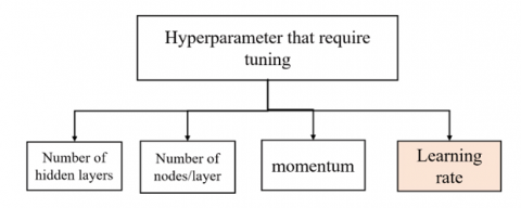
In machine learning, some parameters, such as weights and biases, must be corrected. Both are updated continuously until two conditions are obtained: the optimal error or the reached epoch. In addition, there are also hyperparameter tuning techniques that can be used to improve system performance. Hyperparameter tuning is related to machine learning algorithms, including the number of hidden layers, nodes, or neurons in each layer, momentum, and learning rate [22, 23]. Figure 4 shows the hyperparameters that require tuning so that the network can reach optimal performance.
Figure 4. Hyperparameter that requires tuning
In this study, tuning optimization is made by reducing the learning rate. This activity is carried out when the validation loss does not decrease along with adding epochs. There is a condition for the number of epochs that does not decrease validation loss (2 to 10 epochs). Then, the reduction of the learning rate is carried out [24, 25]. The new learning rate is the old one multiplied by a factor with a specific value (between 0 and 1) [25].
new $l r=l r \times$ factor (2)
where, $l r=$ learning rate$;$ factor $=$ learning rate reduce
A lower limit condition accompanies the reduction in the learning rate. If the lower limit is set to 1×10⁻⁶, then the decrease in the learning rate will stop.
The learning rate needs to be adaptive. One thing that can be done is to reduce the learning rate value. A learning rate that is too large can cause the model to converge more quickly to a suboptimal solution, while a small learning rate value can cause the process to get stuck.
2.8 Output performance
The experiment aims to get the best model of measurement using the confusion matrix. The dataset has three classes, so it uses a multiclass confusion matrix. Performance measurement uses precision, recall, and accuracy. Figure 5 shows the multiclass confusion matrix [26, 27].
Figure 5. Multiclass confusion matrix
From the multiclass confusion matrix, we can get a performance measure of:
(1) Accuracy is calculated as the sum of corrected classifications divided by the total number of classifications.
(2) Precision is calculated as TP/(TP + FP), where TP and FP are the true positive and false positive prediction numbers for the considered class.
(3) Recall calculated as TP and FN are the number of test examples of the considered class.
Any class's total number of test examples would be the sum of the corresponding row (TP+FN). The total number of FNs for a class is the sum of values in the corresponding row, excluding TP. The total number of FPs for a class is the sum of values in the corresponding column, excluding TP. The total number of TNs for a certain class will be the sum of the expected classes' column and row, excluding the class's column and row.
From the Figure 5, we can calculate accuracy, precision, and recall.
Precision class $0=T P_0 /\left(T P_0+E_{1.0}+E_{2.0}\right)$ (3)
Recall class $0=T P_0 /\left(T P_0+E_{0.1}+E_{0.2}\right)$ (4)
Accuracy $=\left(T P_0+T P_1+T P_2\right) /($ All value $)$ (5)
3.1 Experiment environment
The system environment builds on AMD A9-9425 Radeon R5 processor, compute cores 2C+3G 3.10 GHz and 12 GB RAM. We also used Python 3, Google Colaboratory, Tesla T4 GPU, and a 78 GB disk. Tensorflow, Keras, Numpy, Open CV, Seaborn, Scikit Learn, Imblearn, and Streamlit are the libraries used.
3.2 Setting hyperparameter
Table 2. Hyperparameter value
|
Hyperparameter |
Value |
|
learning rate |
0.0001 |
|
epoch |
50 |
|
batch-size |
32 |
|
optimization |
RMSProp |
The system starts by inputting the public dataset into the program. The initial weights use transfer learning weights from imagenet. The hyperparameter value is shown in Table 2. Other hyperparameter values, such as the number of hidden layers, the number of nodes/neurons for each hidden layer, and momentum adjusted to the default of the Inception-V3 architecture. On the other hand, the use of the learning rate was reduced to improve performance results.
3.3 Experimental result
The experiment was carried out by dividing the training and testing data into five parts with 5-fold cross-validation. Four amounts of the data are for training, and the rest for testing. Figure 6 shows a graph of experimental results comparing loss gains from training and validation data. Validation loss is a metric for reducing learning rates. The results show that in each fold, the validation loss is relatively stable at epochs between 20 and 30.
Figure 6 shows information on a decrease in the learning rate. The reduction in each fold varies from epoch 18 in fold 1, epoch 12 in fold 2, epoch 17 in fold 3, epoch 12 in fold 4, and epoch 14 in fold 5. The decrease in the value of the learning rate uses a factor of 0.5. The lower limit of the learning rate is 1×10⁻⁶. Details on the decline in learning rate values and events at certain epochs can be found in Table 3.
Table 3. Reducing the learning rate
|
lr |
Epoch (Intervals) |
||||
|
Fold 1 |
Fold 2 |
Fold 3 |
Fold 4 |
Fold 5 |
|
|
1×10⁻⁴ |
1-17 |
1-11 |
1-16 |
1-11 |
1-13 |
|
5×10⁻⁵ |
18-22 |
12-19 |
17-21 |
12-16 |
14-19 |
|
2.5×10⁻⁵ |
23-27 |
20-24 |
22-26 |
17-23 |
20-26 |
|
1.25 ×10⁻⁵ |
28-32 |
25-29 |
27-31 |
24-28 |
27-31 |
|
6.25×10⁻⁶ |
33-37 |
30-34 |
32-36 |
29-33 |
32-36 |
|
3.125×10⁻⁶ |
38-42 |
35-39 |
37-41 |
34-49 |
37-41 |
|
1.5625×10⁻⁶ |
43-47 |
40-44 |
42-46 |
40-43 |
42-46 |
|
1×10⁻⁶ |
48-50 |
45-50 |
47-50 |
44-50 |
47-50 |
Table 2 shows a decrease in the learning rate value seven times, starting from 1 × 10⁻⁴ to 1×10⁻⁶. The decreasing interval is not the same in each fold, even though when testing initializes the change setting in the form of "patience = 5". This means that if there is an increase in validation loss five times, the learning rate value will automatically decrease by 50%.
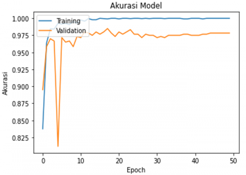
Furthermore, Figure 7 shows a graph of each fold's training and validation accuracy.
(a)
(b)
(c)
(d)
(e)
Figure 6. Validation loss of fold 1 until 5
(a)
(b)
(c)
(d)
(e)
(e)
Figure 7. Training and validation graphs use 5-fold cross-validation
Figure 8 Confusion matrix folds one until fold five. Class 0: adenocarcinoma; 1: squamous cell carcinoma; 2: benign tissue
Table 4. Performance measure of model
|
fold |
epoch |
loss |
valid. loss (%) |
acc. (%) |
valid. acc. (%) |
lr |
|
1 |
33 |
1.86e-07 |
18.61 |
100 |
98.67 |
6.25×10⁻⁶ |
|
2 |
31 |
6.3205e-06 |
17.09 |
100 |
98.67 |
6.25×10⁻⁶ |
|
3 |
44 |
9.8638e-08 |
7.33 |
100 |
99.17 |
1×10⁻⁶ |
|
4 |
18 |
0.0020 |
10.71 |
99.92 |
98.5 |
2.5×10⁻⁵ |
|
5 |
38 |
1.2615e-04 |
9.45 |
100 |
98.83 |
3.125×10⁻⁶ |
Table 5. System Performance
|
|
Precision |
Recall |
Acc. |
||||||
|
Class |
avg. |
Class |
avg. |
||||||
|
0 |
1 |
2 |
0 |
1 |
2 |
||||
|
1 |
98.4 |
100 |
97.5 |
98.6 |
97.5 |
100 |
98.5 |
98.6 |
98.6 |
|
2 |
98.4 |
100 |
98.0 |
98.8 |
98.0 |
99.5 |
98.5 |
98.6 |
98.6 |
|
3 |
98.9 |
100 |
98.5 |
99.1 |
98.5 |
98.5 |
100 |
99.0 |
99.1 |
|
4 |
98.9 |
100 |
98.5 |
98.5 |
96.5 |
100 |
99.0 |
98.5 |
98.5 |
|
5 |
98.4 |
99.5 |
98.8 |
98.8 |
98.0 |
100 |
98.5 |
98.8 |
98.8 |
The experimental results show that validation accuracy gets convergent performance results. Table 4 shows model performance measures (loss, validation loss, accuracy, and validation accuracy) at a particular epoch and learning rate.
Table 4 shows that the highest validation accuracy can be achieved at different epochs. Fold three occurs in epoch 44 of 99.17%. Meanwhile, fold four occurs in epoch 18 with a validation accuracy of 98.5%. Furthermore, Figure 8 shows the confusion matrix of each fold.
Get performance values from Precision, Recall, and Accuracy from the confusion matrix. Table 5 shows the complete performance of the system that has been built.
The experimental results show that the best fold is the 3rd fold, which produces 99.17% accuracy, 99.17% precision, and 99% recall. The amount of training data is 2,400, while the number of testing data is 600. The best validation is in class 1, which is squamous cell carcinoma. The average validation accuracy is 99%.
Based on Figure 8, it can be noted about classification errors. Table 6 shows the number of classification errors in each class.
Experiments show that the class with the best recognition is class 1 squamous cell carcinomas. Meanwhile, the class with the lowest classification results is class 0 adenocarcinoma.
Next, compare the experimental results with previous studies. Table 6 shows a comparison with existing previous research.
Comparisons can be made in the author's articles [13, 14], and the proposed method. Table 7 shows the improvements in performance measures, accuracy of 99.17%, precision of 99.17%, and recall of 99%.
Classification has been carried out using transfer learning inception-v3 with learning rate tuning. To produce varied models, 5-fold cross-validation is used. Each fold creates a model to be used in the testing stage. Testing results show that fold-3 has the best accuracy. Experiments show that the technique used can improve classification results.
Table 6. Number of classification error
|
Class |
Fold |
Classification Error |
||||
|
1 |
2 |
3 |
4 |
5 |
||
|
0 |
5 |
4 |
3 |
7 |
4 |
23 |
|
1 |
0 |
1 |
0 |
0 |
0 |
1 |
|
2 |
3 |
3 |
2 |
2 |
3 |
13 |
Table 7. Proposed system vs. previous research
|
Reference |
Method |
Dataset |
Acc. |
Prec. |
Rec. |
|
[9] |
Deep CNN |
Original |
71.1 |
- |
- |
|
[10] |
DenseNet121 |
JSRT |
84.02 |
85.34 |
82.71 |
|
[11] |
SVM |
- |
- |
- |
- |
|
[12] |
VGG16 |
ACDC@LUNGHP |
75.41 |
- |
- |
|
[13] |
CNN gamma correction |
LC25000 |
87.16 |
86.67 |
87.00 |
|
[14] |
ResNet18 |
LC25000 |
98.82 |
- |
- |
|
Proposed |
Transfer learning Inception-v3 with reduced lr |
LC25000 |
99.17 |
99.17 |
99.00 |
This research consists of two steps: preprocessing and classification. Preprocessing aims to prepare the data better and reduce the size of the image. Meanwhile, classification using deep learning CNN has many factors that contribute to getting the best results. Each trial carried out has a hypothesis to improve performance. CNN has an Artificial Neural Network (ANN) backbone uses initial optimization with backpropagation. Next is optimization using gradient descent to update the weights by minimizing the loss function. Finally, there is learning rate tuning, which aims to improve performance.
In this study, several factors that contribute to producing good performance, including:
Preprocessing has been carried out in previous research to produce the best gamma value 1.2 [7]. Furthermore, the system performs training on the data using CNN Inception-v3. As explained in sub-chapter 3.4, the advantages of inception version 3 are factorization with smaller convolutions, asymmetrical factorization, auxiliary classifier, and grid-size reduction. Better than the previous version.
The system uses transfer learning from ImageNet weights. High specifications constrained the system being run. The number of datasets that should have been 15,000 was cut to just 3,000. Of course, this data reduction affects the existing training process. However, transfer learning is the best solution because it utilizes a model that has been previously trained, even though the dataset is limited. Furthermore, optimization using gradient descent RMSProp.
As a deep learning method, CNN requires more data and higher computation than traditional machine learning methods. CNN has hyperparameters: batch size, epoch, and learning rate. Determination of hyperparameter values is carried out through experiments. For batch size, the system can process data at one time. The larger the batch-size value, the faster the iterations and epochs. If the hardware has high specifications, choosing a high batch-size value is recommended. Meanwhile, the learning rate is the rate of learning. If the learning rate value is high, it will converge quickly, and overfitting will occur; if the value is too low, the process will stop at sub-optimal.
The following components that affect system results are hyperparameters, such as learning rate, epoch, and batch size. The initialized epoch is 50. The batch size is 32. The higher the epoch value means that there are more iterations of learning. However, this does not guarantee increased performance. There must be more consistency and a good epoch value for image classification. The researcher must have an experiment to get the appropriate epoch. The batch size is the system's ability to process data simultaneously. We can initialize a batch size with a higher value if we have high computer specifications. Generally, batch size has a value of 2n, such as 16,32, 64, or 128.
The last component that supports the performance of the classification system is the decreasing learning rate. The learning rate can be reduced as the epoch increases. The learning rate can be decreased if validation loss increases five times (patience = '5'). The experiment shows an improvement in performance measures.
Decreasing the learning rate can help optimize validation accuracy performance values. Table 3 shows a decrease in the learning rate value from an improvement in the validation accuracy value from the 5-fold experiment. Validation accuracy results start from 98.5% to 99.17%. A validation accuracy value of 99.17% was obtained when the learning rate value was 1×10⁻⁶.
The research that has been carried out has limitations, including the fact that the Inception-v3 architectural model is complicated to understand because of the large number of exception series with different filter values. Apart from that, the dataset used for the experiment only partially uses part of the dataset due to computational limitations.
Research has been carried out on the classification of lung cancer into three classes: adenocarcinoma, squamous cell carcinoma, and benign tissue. The research results can then be used for consideration or a second opinion regarding lung cancer screening stages.
In this study, lung cancer has been classified using inception-v3. The preprocessing with gamma correction 1.2. The classification using CNN with transfer learning from the pre-trained network using ImageNet weights. Hyperparameter initialization includes epoch 50, batch size 32, and a reduced learning rate if there is an increase in validation loss. The experiment uses 5-fold cross-validation. The validation results show 99.17% accuracy, 99.17% precision, and 99% recall.
This research has limitations: using a dataset of only 3,000 of the 15,000 images in the lung cancer dataset. The architectural model used is quite complicated to understand because of the many differences in the size and number of filters of the inception block. Apart from that, hyperparameter tuning is only limited to the learning rate.
Future research can use all the images contained in the dataset. The architectural model can use simpler architecture and computing such as mobile net or a hybrid between CNN architectures. Meanwhile, hyperparameter tuning can use randomized search to get the optimal value for each variable.
Research can be carried out experimentally using other secondary and even primary hospital data. This research can then be developed into an applied type in collaboration with pulmonary doctors and hospitals to determine the effectiveness of the resulting prototype.
This work was supported by Penelitian Program Kompetitif Nasional & Penugasan scheme Penelitian Dasar Kompetitif Nasional 2023 from the Indonesia Ministry of Education, Culture, Research and Technology.
[1] Kurniyanto (2022). Bagaimana kanker paru dapat diketahui lebih awal sebelum stadium lanjut? https://yankes.kemkes.go.id/view_artikel/1550/bagaimana-kanker-paru-dapat-diketahui-lebih-awal-sebelum-stadium-lanjut.
[2] (2018). Buku Pedoman Pengendalian Faktor Risiko Kanker Paru_ Tahun 2018. https://p2ptm.kemkes.go.id/ dokumen-ptm/buku-pedoman-pengendalian-faktor-risiko-kanker-paru_-tahun-2018.
[3] Yuan, L., Chen, D., Chen, Y.L., et al. (2021). Florence: A new foundation model for computer vision. arXiv preprint arXiv:2111.11432. https://doi.org/10.48550/arXiv.2111.11432
[4] Esteva, A., Chou, K., Yeung, S., Naik, N., Madani, A., Liu, Y., Topol, E., Dean, J., Socher, R. (2021). Deep learning-enabled medical computer vision. NPJ digital medicine, 4(1): 5. https://doi.org/10.1038/s41746-020-00376-2
[5] Möller, D. (2023). Machine learning and deep learning. Guide to Cybersecurity in Digital Transformation, pp. 347-384. https://doi.org/10.1007/978-3-031-26845-8_8
[6] Niu, Z., Zhong, G., Yu, H. (2021). A review on the attention mechanism of deep learning. Neurocomputing, 452: 48-62. https://doi.org/10.1016/j.neucom.2021.03.091
[7] Dong, S., Wang, P., Abbas, K. (2021). A survey on deep learning and its applications. Computer Science Review, 40: 100379. https://doi.org/10.1016/j.cosrev.2021.100379
[8] Tan, C., Sun, F., Kong, T., Zhang, W., Yang, C., Liu, C. (2018). A survey on deep transfer learning. In Artificial Neural Networks and Machine Learning–ICANN 2018: 27th International Conference on Artificial Neural Networks, Rhodes, Greece, pp. 270-279. https://doi.org/10.1007/978-3-030-01424-7_27
[9] Teramoto, A., Tsukamoto, T., Kiriyama, Y., Fujita, H. (2017). Automated classification of lung cancer types from cytological images using deep convolutional neural networks. BioMed Research International, 2017: 4067832. https://doi.org/10.1155/2017/4067832
[10] Ausawalaithong, W., Thirach, A., Marukatat, S., Wilaiprasitporn, T. (2018). Automatic lung cancer prediction from chest X-ray images using the deep learning approach. In 2018 11th biomedical engineering international conference (BMEiCON), Chiang Mai, Thailand, pp. 1-5. https://doi.org/10.1109/BMEiCON.2018.8609997
[11] Rahane, W., Dalvi, H., Magar, Y., Kalane, A., Jondhale, S. (2018). Lung cancer detection using image processing and machine learning healthcare. In 2018 International Conference on Current Trends towards Converging Technologies (ICCTCT), Coimbatore, India, pp. 1-5. https://doi.org/10.1109/ICCTCT.2018.8551008
[12] Šarić, M., Russo, M., Stella, M., Sikora, M. (2019). CNN-based method for lung cancer detection in whole slide histopathology images. In 2019 4th International Conference on Smart and Sustainable Technologies (SpliTech), Split, Croatia, pp. 1-4. https://doi.org/10.23919/SpliTech.2019.8783041
[13] Setiawan, W., Suhadi, M. M., Pramudita, Y.D. (2022). Histopathology of lung cancer classification using convolutional neural network with gamma correction. Communications in Mathematical Biology and Neuroscience, 2022: 81.
[14] Wahid, R.R., Nisa, C., Amaliyah, R.P., Puspaningrum, E.Y. (2023). Lung and colon cancer detection with convolutional neural networks on histopathological images. AIP Conference Proceedings, 2654(1): 020020. AIP Publishing. https://doi.org/10.1063/5.0114327
[15] Borkowski, A.A., Bui, M.M., Thomas, L.B., Wilson, C.P., DeLand, L.A., Mastorides, S.M. (2019). Lung and colon cancer histopathological image dataset (lc25000). arXiv preprint arXiv:1912.12142. https://doi.org/10.48550/arXiv.1912.12142
[16] Garg, S., Garg, S. (2020). Prediction of lung and colon cancer through analysis of histopathological images by utilizing Pre-trained CNN models with visualization of class activation and saliency maps. In Proceedings of the 2020 3rd Artificial Intelligence and Cloud Computing Conference, Kyoto, Japan, pp. 38-45. https://doi.org/10.1145/3442536.3442543
[17] Khatami, A., Babaie, M., Khosravi, A., Tizhoosh, H.R., Nahavandi, S. (2018). Parallel deep solutions for image retrieval from imbalanced medical imaging archives. Applied Soft Computing, 63: 197-205. https://doi.org/10.1016/j.asoc.2017.11.024
[18] Szegedy, C., Vanhoucke, V., Ioffe, S., Shlens, J., Wojna, Z. (2016). Rethinking the inception architecture for computer vision. In 2016 IEEE Conference on Computer Vision and Pattern Recognition (CVPR), Las Vegas, NV, USA, pp. 2818-2826. https://doi.org/10.1109/CVPR.2016.308
[19] Kornblith, S., Shlens, J., Le, Q.V. (2019). Do better imagenet models transfer better? In 2019 IEEE/CVF Conference on Computer Vision and Pattern Recognition (CVPR), Long Beach, CA, USA, pp. 2656-2666. https://doi.org/10.1109/CVPR.2019.00277
[20] Huh, M., Agrawal, P., Efros, A.A. (2016). What makes ImageNet good for transfer learning? arXiv preprint arXiv:1608.08614. https://doi.org/10.48550/arXiv.1608.08614
[21] Javanmardi, S., Ashtiani, S.H.M., Verbeek, F.J., Martynenko, A. (2021). Computer-vision classification of corn seed varieties using deep convolutional neural network. Journal of Stored Products Research, 92: 101800. https://doi.org/10.1016/j.jspr.2021.101800
[22] Amirabadi, M.A., Kahaei, M.H., Nezamalhosseini, S. A. (2020). Novel suboptimal approaches for hyperparameter tuning of deep neural network [under the shelf of optical communication]. Physical Communication, 41: 101057. https://doi.org/10.1016/j.phycom.2020.101057
[23] Jiang, X., Xu, C. (2022). Deep learning and machine learning with grid search to predict later occurrence of breast Cancer metastasis using clinical data. Journal of Clinical Medicine, 11(19): 5772. https://doi.org/10.3390/jcm11195772
[24] ReduceonPlateau. https://pytorch.org/docs/stable/generated/torch.optim.lr_scheduler.ReduceLROnPlateau.html.
[25] ReduceLROnPlateau. https://keras.io/api/callbacks/reduce_lr_on_plateau/#:~:text=ReduceLROnPlateau class&text=Reduce learning rate when a,the learning rate is reduced.
[26] Markoulidakis, I., Kopsiaftis, G., Rallis, I., Georgoulas, I. (2021). Multi-class confusion matrix reduction method and its application on net promoter score classification problem. In Proceedings of the 14th PErvasive Technologies Related to Assistive Environments Conference, Corfu, Greece, pp. 412-419. https://doi.org/10.1145/3453892.3461323
[27] Haghighi, S., Jasemi, M., Hessabi, S., Zolanvari, A. (2018). PyCM: Multiclass confusion matrix library in Python. Journal of Open Source Software, 3(25): 729. https://doi.org/10.21105/joss.00729