Jafar Abukhait![]()
© 2024 The author. This article is published by IIETA and is licensed under the CC BY 4.0 license (http://creativecommons.org/licenses/by/4.0/).
OPEN ACCESS
A significant challenge for Photovoltaic (PV) power systems is the accumulation of dust on solar panels, particularly prevalent in desert areas. Dust accumulation on solar panels cause a high degradation in the output power and thus, solar panels should be monitored and cleaned continuously to keep their efficiency high. Automating the inspection of solar panels can serve as a viable alternative of human inspection due to the impact of labor expenses and human difficulties on decision-making on such an environment. In this work, we are proposing a computer vision approach that is capable of inspecting solar panels and determines its condition in terms of dust accumulation. The proposed approach aims to prove the capability of dust detection on distinct panels by means of visible light imaging and computer vision techniques. It deploys both gray level co-occurrence matrix (GLCM) textural features and local binary patterns (LBP) of solar panels’ images in addition to support vector machine (SVM) to build a classification model for this purpose. The proposed approach has been tested on images of solar panels that suffer from moderate and heavy accumulation of desert sands and dusts. The experimental findings successfully illustrated the effectiveness of the proposed feature description and the overall dust detection approach of solar panels with an accuracy of 94.3%.
dust detection, gray level co-occurrence matrix, local binary pattern, photovoltaic panels, support vector machine
Automated inspection techniques have been widely adopted in the industry sector in the last two decades to detect defect regions on solar panels or to identify the defect type and its existence on these panels. These defects are formulated, from the perspective of image processing, as local textural features [1]. Automated inspection of solar panels is an alternate of human visual inspection, where real-time feedback is required when a certain defect occurs because of labor costs and human distraction that affect the decision [2]. Solar panels are devices engineered to transform sunlight into electricity, capturing solar energy and converting it into usable electrical power.
In Middle East countries, although solar radiation intensity is very high, desert sands and dust accumulation represent a natural barrier that can significantly impair their capacity to generate energy [3]. Over time, dust, grime, and various particles settle on the panel surfaces, forming a fine layer that hampers sunlight from reaching the photovoltaic cells. This layer diminishes the panels' efficiency in absorbing and transforming solar energy into electricity. Consequently, the Photovoltaic (PV) system's energy output declines, resulting in a substantial reduction in energy production [4, 5]. Consistent monitoring and cleaning are imperative to mitigate the detrimental impacts of dust accumulation, ensuring that solar panels sustain their optimal functionality, thereby maximizing their contribution to clean and sustainable energy generation.
Existing technologies for dust detection range from manual inspection to automated systems utilizing drones, robots, or sensors. Manual inspections are cost-effective but time-consuming and often impractical for large-scale installations. Automated methods relying on vision technology offer advantages such as increased efficiency, accuracy, early detection of defects, and reduced labor costs [6]. However, they may come with disadvantages including initial investment costs, maintenance requirements, and potential limitations due to lighting conditions and variations in surface texture detecting certain types of contaminants or in challenging environmental conditions [7]. In addition, current proposed dust detection techniques have many shortcomings including short-range acquisition and considering moderate and heavy dust densities on solar panels in desert areas. Nevertheless, despite these limitations, solar panel inspections remain indispensable for detecting dust accumulation, optimizing performance, initiating cleaning actions, and ensuring the secure and efficient operation of PV systems. Striking a balance between effectiveness, cost, and practicality is essential in implementing a reliable dust detection strategy for PV panels.
This paper proposes a computer vision approach to inspect the solar panel condition in terms of dust accumulation. The proposed approach has the ability to classify automatically solar panels to clean and dust-accumulated regardless of lighting conditions and texture variations. The proposed approach introduces a feature description by the fusion of both gray level co-occurrence matrix (GLCM) textural features and uniform local binary patterns (LBP). This approach can be integrated with automated monitoring and cleaning systems of solar panels that combine technologies such as an unmanned aerial vehicle (UAV) and digital imaging. This work has the following contributions:
Furthermore, the paper is structured as follows: Section 2 demonstrates a review of prior research. Section 3 presents a mathematical background of the computer vision and artificial intelligence techniques used in this work. The proposed dust detection approach is presented in Section 4 while the experimental findings along with performance measures are demonstrated in Section 5. Finally, Section 6 provides the conclusions.
Various methodologies outlined in the literature have been employed to analyze the influence of environmental factors on solar photovoltaic output, either through experimental studies or the creation of predictive models. Previous research has investigated the effects of dust on Photovoltaic (PV) power systems. The findings revealed a substantial decrease in solar panel efficiency when exposed to dust particles proportion to dust sample weight [8, 9]. Other works have showed experimentally the relationship between dust quantities and power degradation [10-12]. They revealed that moderate and heavy accumulation in desert areas has severe effect on power generation in comparison with light or typical accumulation.
Automated dust detection techniques rely either on infrared imaging or visible light imaging [13]. In the study by Phoolwani et al. [14, 15], dust accumulation has been estimated based on infrared imaging in which heat concentration on solar panels can be identified.
Visible light imaging was recently suggested by several researchers to mimic the behavior of human in identifying dust accumulation on solar panels. In the study by Abuqaaud and Ferrah [16], a computer vision technique for identifying soil and dust on PV surfaces has been proposed. The technique relies on extracting features using the GLCM and accomplishing classification through a linear classifier. The proposed technique was applied on images of PV panels fixed on a stand and achieved 82 % recognition rate.
In the study by Tribak and Zaz [17], the researchers introduced an image processing-centered system designed to gauge the quantity of dust collected on the surface of solar panels. They utilized small, plasticized paper as an indicator for image processing.
Unluturk et al. [18] used artificial light source to estimate three different levels of dust accumulation on the PV surface. Features were obtained based on GLCM and classification was achieved using Artificial Neural Networks (ANN) to determine dust level. The proposed system has achieved 96.86 % accuracy.
In the study by Onim et al. [19], a convolutional neural network model named “SolNet” was developed that has the ability to detect the dust accumulation on solar panels. The proposed model has been trained and tested on a dataset of 2231 images. These images have been acquired from short range and the have light and typical dust accumulation. The proposed model has been proved with and accuracy of 98.2%.
In conclusion, the literature demonstrates several attempts to implement automated vision-based dust detection methodologies from infrared cameras. Dust detection from images acquired under visible light is an ongoing domain that has to address several shortcomings such as: 1) the acquisition methodology which is currently achieved in most cases in parallel to solar panels, from short range, or under artificial light; 2) current datasets of digital images have small portion of dust accumulation as opposed to real situations in desert areas in which moderate and heavy accumulation occurs; 3) current detection techniques do not deploy textural features on solar panel images which is expected to perform efficiently. These shortcomings have inspired this work which aims to implement and prove a computer vision approach for dust accumulation.
3.1 Gray level co-occurrence matrix
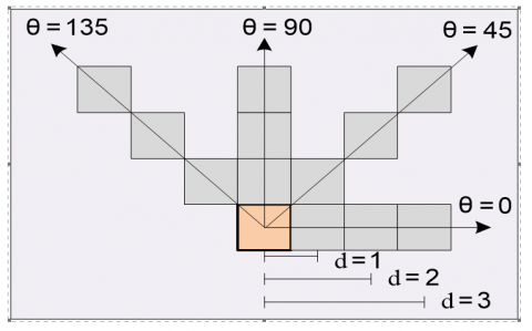
The gray level co-occurrence matrix (GLCM) is typically deployed to extract global textural features of an image. It is defined as the distribution of co-occurring gray levels at a given offset: direction (θ) and distance (d). The relative frequencies of two neighboring pixels, one with gray level i and the other with gray level j, are calculated from the quantized image to construct the co-occurrence matrix Pij. This co-occurrence matrix (Pij) can be calculated with different values of d such as: 1, 2, and 3 and different values of θ such as: 0, 45, 90, and 135 as shown in Figure 1.
Figure 1. GLCM with different offsets
Several textural features can be derived from the co-occurrence matrix Pij, including Energy, Contrast, Correlation, Homogeneity, Entropy, Autocorrelation, Dissimilarity, and Cluster Shade [20]. The following equations define some of these features where p(i, j) is the (i, j)th cell in the co-occurrence matrix, µx and µy are the mean values for rows and columns of the matrix, σx and σy are the standard deviation values for rows and columns of the matrix, Ng is the number of gray levels in the quantized image [20-22]:
$\mu_x=\sum_i \sum_j i \cdot p(i, j)$ (1)
$\mu_y=\sum_i \sum_j j \cdot p(i, j)$ (2)
$\sigma_{\mathrm{x}}=\sum_{\mathrm{i}} \sum_{\mathrm{j}}\left(\mathrm{i}-\mu_{\mathrm{x}}\right)^2 \cdot \mathrm{p}(\mathrm{i}, \mathrm{j})$ (3)
$\sigma_y=\sum_i \sum_j\left(i-\mu_y\right)^2 \cdot p(i, j)$ (4)
The textural features are defined as follows [20-22]:
$\mathrm{f}_1=\sum_{\mathrm{i}} \sum_{\mathrm{j}} \mathrm{p}(\mathrm{i}, \mathrm{j})^2$ (5)
$f_2=\sum_{n=0}^{N_g-1} n^2\left\{\sum_{i=1}^{N_g} \sum_{\substack{j=1 \\|i-j|=n}}^{N_g} p(i, j)\right\}$ (6)
$\mathrm{f}_3=\frac{\sum_{\mathrm{i}} \sum_{\mathrm{j}}(\mathrm{ij}) \mathrm{p}(\mathrm{i}, \mathrm{j})-\mu_{\mathrm{x}} \mu_{\mathrm{y}}}{\sigma_{\mathrm{x}} \sigma_{\mathrm{y}}}$ (7)
$f_4=\sum_i \sum_j \frac{1}{1+(i-j)^2} p(i, j)$ (8)
$f_5=-\sum_i \sum_j p(i, j) \log (p(i, j))$ (9)
$\mathrm{f}_6=\sum_{\mathrm{i}} \sum_{\mathrm{j}}(\mathrm{ij}) \cdot \mathrm{p}(\mathrm{i}, \mathrm{j})$ (10)
$f_7=\sum_i \sum_j|i-j| \cdot p(i, j)$ (11)
$f_8=\sum_i \sum_j\left(i+j-\mu_x-\mu_y\right)^3 \cdot p(i, j)$ (12)
3.2 Local binary pattern
Local Binary Pattern (LBP) is a feature extraction operator designed for grayscale images that is invariant to both rotation and scale [23, 24]. It aims to capture local texture characteristics within an image. To compute the LBP value for a specific pixel location (Xc, Yc), a comparison is made between a pixel value and its neighbors. If the neighbor pixel value surpasses the target pixel value, it is labeled as 1; otherwise, it is labeled as 0. The number of neighboring pixels considered in this comparison can range from 4, 8, 12, 16, to 24. When comparing with the eight immediate neighboring pixels, this process yields an 8-bit binary code. This binary code can then be converted into a decimal value, which is subsequently assigned as the new pixel value for the central pixel, as shown in Figure 2.
Figure 2. Schematic of LBP with eight pixel surroundings
LBP can be computed according to Eq. (13) as:
$\operatorname{LBP}_{\mathrm{P}}\left(\mathrm{X}_{\mathrm{c}}, \mathrm{Y}_{\mathrm{c}}\right)=\sum_{\mathrm{p}=0}^{\mathrm{P}-1} \mathrm{~S}\left(\mathrm{~g}_{\mathrm{p}}-\mathrm{g}_{\mathrm{c}}\right) 2^{\mathrm{p}}$ (13)
where, ɡc is the gray level of the centered pixel, ɡp is the gray value of neighboring pixels, P is the number of surrounding pixels, and S is a function defined as:
$S(x)= \begin{cases}0, & x<0 \\ 1, & x \geq 0\end{cases}$ (14)
The LBPp operator produces 2P different local binary patterns. Rotation-invariant LBP can be computed according to Eq. (15) as:
$\mathrm{LBP}_{\mathrm{P}}^{\mathrm{ri}}=\min \left\{\operatorname{ROR}\left(\mathrm{LBP}_{\mathrm{p}}, \mathrm{i}\right) \mid \mathrm{i}=0,1, \ldots \ldots, \mathrm{P}-1\right\}$ (15)
where, ROR(x,i) function applies a circular right shift on the P-bit number I times and thus; achieving 36 unique rotation invariant local binary patterns in case of LBPP. These Rotation-invariant LBP describe bright spots, dark spots, and edges [25].
In the study by Ojala et al. [23], an enhanced version of the Local Binary Pattern (LBP) is introduced, which incorporates a uniformity measure denoted as “U.” This measure is defined as the count of spatial transitions, representing bitwise changes from 0 to 1 or vice versa, within the local binary pattern. For instance, a pattern like “111111112” is assigned a U value of 0, while a pattern like “000011112” is given a U value of 2. This uniformity measure serves to categorize local binary patterns into two distinct groups: “uniform” patterns, which are intrinsic properties of texture and exhibit a U value of no more than 2, and “nonuniform” patterns. The formula for the modified LBP is then expressed as follows:
$\operatorname{LBP}_{\mathrm{P}}^{\mathrm{riu} 2}=\left\{\begin{array}{lr}\sum_{\mathrm{p}=0}^{\mathrm{P}-1} \mathrm{~S}\left(\mathrm{~g}_{\mathrm{p}}-\mathrm{g}_{\mathrm{c}}\right) & \text { if } \mathrm{U}\left(\mathrm{LBP}_{\mathrm{P}}\right) \leq 2 \\ \mathrm{P}+1 & \text { otherwise }\end{array}\right.$ (16)
This definition results in the creation of P+1 uniform patterns and 1 nonuniform pattern. The nonuniform pattern encompasses all patterns with a U value greater than 2. As a result, the total number of LBP patterns is reduced to P+2 patterns. In case of P=8, nine uniform patterns and one Non-uniform pattern, as shown in Figure 3, would be produced.
Figure 3. Examples of LBP8 patterns: (a) The nine Uniform patterns and (b) Non-uniform patterns
The histogram of LBP patterns, collected across a surface image, serves as the feature descriptor for characterizing surface texture. In the study by Ojala et al. [23], the researchers came to the conclusion that the histogram of uniform patterns outperforms histograms based on other LBP pattern types in terms of discrimination capabilities.
3.3 Support vector machine
The Support Vector Machine (SVM) is essentially a statistical binary classifier that employs kernel functions. When employing a sigmoid kernel function, an SVM shows similarities to the response of a two-layer feedforward neural network. However, SVM demonstrates greater efficiency than neural networks when dealing with intricate problems involving extensive datasets and high dimensionality, and it is adept at mitigating overfitting concerns [26-28].
The core concept of SVM is to identify the optimal hyperplane that maximizes the margin between the hyperplane and the closest data points from both classes. SVM can be formulated as follows:
If input space is: {x1, x2, x3, …, xn}
and output space is: $y \in\{-1,1\}$
The hyperplane that separates the two classes is expressed as [28-30]:
$\overrightarrow{\mathrm{w}} \cdot \overrightarrow{\mathrm{x}}+\mathrm{b}=0$ (17)
here, w (weight) denotes the orthogonal vector defining the orientation of the hyperplane, while b (bias) represents the distance from the origin to the hyperplane.
Training instances must satisfy:
$\overrightarrow{\mathrm{w}} \cdot \overrightarrow{\mathrm{x}}+\mathrm{b} \geq 1$ for $\mathrm{y}=+1$ (18)
$\overrightarrow{\mathrm{w}} \cdot \overrightarrow{\mathrm{x}}+\mathrm{b} \leq-1$ for $\mathrm{y}=-1$ (19)
The previous inequalities are merged to obtain:
$y(\vec{w} \cdot \vec{x}+b)-1 \geq 0$ (20)
This can be formulated as:
$\operatorname{maximize} \frac{2}{\|\mathrm{w}\|}$ or minimize $\frac{1}{2}\|\mathrm{w}\|^2$ (21)
Such that: $\mathrm{y}(\overrightarrow{\mathrm{w}} \cdot \overrightarrow{\mathrm{x}}+\mathrm{b})-1 \geq 0$
For solving Eq. (21), a Lagrange multiplier is deployed and it yields:
$\min L_p \equiv \frac{1}{2}\|\vec{w}\|^2-\sum_{i=1}^l \alpha_i y_i\left(\vec{w} \cdot \overrightarrow{x_1}+b\right)+\sum_{i=1}^l \alpha_i$ (22)
Such that αi ≥ 0 where α is the Lagrange multiplier.
The result is a decision function of Lagrange multipliers α and bias (b) for test instance xt:
$y_t=\sum_{i=1}^1\left(\alpha_i y_i<\overrightarrow{x_1} \cdot \overrightarrow{x_t}>+b\right)$ (23)
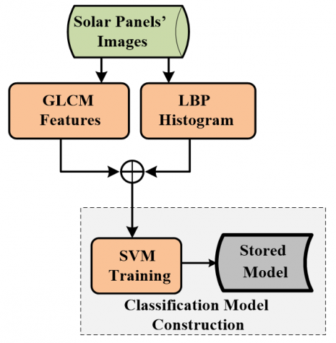
The dust detection approach, as shown in Figure 4, consists of three stages:
Figure 4. Diagram of the dust detection approach
4.1 Data acquisition
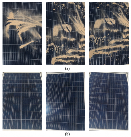
In this stage, solar panel images were acquired under visible light from 10:00 am to 4:00 pm using RGB camera with a 20 MP resolution. These images simulate the real environmental conditions of automated dust detection systems as they were captured under both low and high lighting conditions in sunny and cloudy days. The image acquisition was performed manually using digital cameras mounted on Selfie stick with a height range between 1.5-4 m which could be the real height of robotic arm in such systems. Dust-accumulated images were increased by applying sand and dust accumulation artificially. Different levels of dust accumulation were considered ranging from moderate to severe. Finally, all images were resized to a resolution of 650 × 875 pixels and cropped manually to achieve distinct image for each solar panel. Figure 5 shows sample images of clean and dust-accumulated solar panels.
Figure 5. Sample images of solar panels with: (a) Accumulated dust and (b) Clean condition
4.2 Feature description
In this stage, feature descriptors of solar panel images are extracted for both clean and dust-accumulated panels. The inputs to this stage are single solar panel images which were obtained after manual preprocessing and cropping.
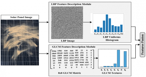
This stage comprises two modules depicted in Figure 6: the Local Binary Pattern (LBP) module and the Gray-level Co-occurrence Matrix (GLCM) module. Each module takes a gray scale image as input and generates a distinct feature descriptor for the image as output. The culmination of both feature descriptors extracted from these modules involves fusing and concatenating them to form a unified feature descriptor. This singular descriptor encapsulates the intricate shape and pattern attributes of the solar panel image. The fusion process merges the local features of LBP with the global features of GLCM, culminating in an optimized descriptor that encapsulates the essence of the solar panel image.
4.2.1 LBP feature description module
This module generates a feature vector (FV) by applying the LBP operator on the solar panel image. A rotation-invariant LBP with eight pixel surroundings has been deployed on each surface image (as demonstrated on sub-section 3.2) to generate a LBP image which describes bright spots, dark spots, and edges. Applying the uniformity measure (U), LBP patterns would be categorized to ‘Uniform’ patterns and ‘Non-uniform’ ones. This would produce nine uniform patterns and one Non-uniform pattern. The final step in this stage is to compute the histogram of LBP uniform patterns. This histogram would have ten bins including the nine uniform patterns and one pin for all other Non-uniform patterns such as:
$\mathrm{FV}$ of $\mathrm{LBP}=\left[\mathrm{U}_0, \mathrm{U}_1, \mathrm{U}_2, \mathrm{U}_3, \mathrm{U}_4, \mathrm{U}_5, \mathrm{U}_6, \mathrm{U}_7, \mathrm{U}_8, \mathrm{NU}\right]$ (24)
4.2.2 GLCM feature description module
This module generates a feature vector (FV) by computing the GLCM for the solar panel image. The image is initially scaled to eight gray levels and then; the co-occurrence matrix Pij is computed with direction (θ=0o) and distance (d=1). Eight textural features are extracted (as demonstrated on sub-section 3.1) from the GLCM matrix denoted as Pij.
These features are: Energy (f1), Contrast (f2), Correlation (f3), Homogeneity (f4), Entropy (f5), Autocorrelation (f6), Dissimilarity (f7), and Cluster Shade (f8). Finally, a feature vector of GLCM is constructed from these features such as:
$\mathrm{FV}$ of $\mathrm{GLCM}=\left[\mathrm{f}_1, \mathrm{f}_2, \mathrm{f}_3, \mathrm{f}_4, \mathrm{f}_5, \mathrm{f}_6, \mathrm{f}_7, \mathrm{f}_8\right]$ (25)
Finally, in this stage, a feature descriptor of length 18 is constructed by combining the ten histogram pins of LBPs (nine uniform LBPs and one non-uniform LBP) and the eight textural features of GLCM. The format of the feature vector would be:
$\begin{gathered}\mathbf{F V}=\left[\mathrm{U}_0, \mathrm{U}_1, \mathrm{U}_2, \mathrm{U}_3, \mathrm{U}_4, \mathrm{U}_5, \mathrm{U}_6, \mathrm{U}_7, \mathrm{U}_8, \mathrm{NU}, \mathrm{f}_1, \mathrm{f}_2,\right. \left.\mathrm{f}_3, \mathrm{f}_4, \mathrm{f}_5, \mathrm{f}_6, \mathrm{f}_7, \mathrm{f}_8\right]\end{gathered}$ (26)
4.3 Inspection model construction
This module constructs a classification model for each solar panel image based on the feature vector produced in the previous stage. Linear SVM is trained on clean and dust-accumulated solar panel images. The SVM classifier is used in its original binary architecture since we have a classification problem of two classes. Tens of images were deployed for training and validating the model. These images were labeled previously by a human expert.
The training data are labeled as: \begin{aligned} & \left.\quad \vec{x}_i, y_i\right\} \quad \text { where } i=1, \ldots \ldots, n ; y_i \in \{1,-1\} ; \vec{x}_i \in\left\{\mathfrak{R}^d\right\}\end{aligned}, $\vec{x}_i$ is the feature vector, yi is the class which represents the status of solar panel in terms of dust accumulation and could be 1 (if clean) or -1 (if dust-accumulated), i is the total number of training instances, and d is the length of the feature vector.
The hyperplane that separates the two classes is expressed as:
$\vec{w} \cdot \vec{x}+b=0$ (27)
where, w (weight) denotes the orthogonal vector defining the orientation of the hyperplane, while b (bias) represents the distance from the origin to the hyperplane.
Figure 6. Feature description modules
Several performance metrics were adopted to measure the classification performance. These metrics are Precision (P), Recall (R), Accuracy, and F1 Score which formulated mathematically as:
$P=\frac{T_p}{T_P+F_P}$ (28)
$R=\frac{T_p}{T_P+F_n}$ (29)
Accuracy $=\frac{T_p+T_n}{T_P+F_P+T_n+F_n}$ (30)
F1 Score $=\frac{2 * P * R}{P+R}$ (31)
where, Tp is the number of correctly predicted dust-accumulated solar panels, Tn is the number of correctly predicted clean solar panels, Fp is the number of incorrectly predicted dust-accumulated solar panels, and Fn is the number of incorrectly predicted clean solar panels.
The proposed approach for inspecting solar panels’ conditions in terms of dust accumulation has undergone validation using images of both clean and dust-accumulated solar panels. These images were captured using a camera and adjusted to a 650 × 870 pixel scale through numerical fractioning to counteract object distortion. Implemented within MATLAB software running on a 2.4-GHz i3 CPU, this inspection approach utilized a dataset comprising 213 solar panel images for both training and testing phases. We have allocated 75% of the images for the training set and 25% for the testing set. Table 1 shows the exact division of dataset images among the classification phases and the solar panels’ conditions.
Table 1. Solar panel images dataset division
|
|
Clean Solar Panel |
Dust-Accumulated Solar Panel |
Total Number of Images |
|
Number of Training Images |
80 |
80 |
160 |
|
Number of Testing Images |
30 |
23 |
53 |
|
Total Number of Images |
110 |
103 |
213 |
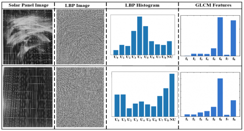
Each solar panel image in the dataset has had its feature descriptor extracted, becoming its representative signature. This descriptor is a combination of the histogram of uniform LBP patterns and eight textural features computed from the GLCM.
In Figure 7, examples of clean and dust-accumulated solar panel images are displayed alongside the features extracted from both the LBP Uniforms histogram and GLCM textural analysis. It is apparent that both LBP and GLCM feature descriptors are different for clean and dust-accumulated solar panels.
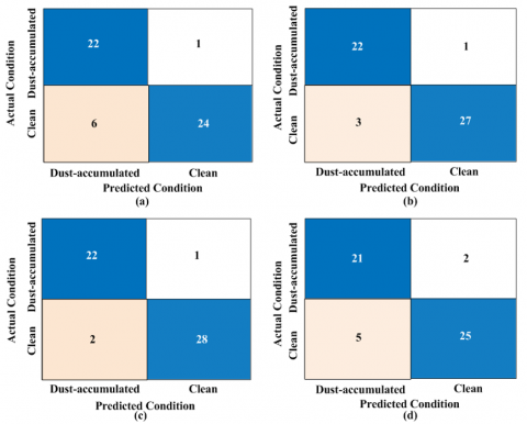
The extracted features were fed to implement a binary classification model using linear support vector machine. This model aims to classify solar panels either to clean or dust-accumulated condition. Four experiments were implemented in the classification stage. The first experiment was implemented based on all Uniform and Non-uniform patterns of LBP. The second experiment was implemented by concatenating the ten LBP patterns and the eight GLCM textural features. The third and fourth experiments were implemented by adopting Recursive Feature Elimination (RFE) with number of features equals 15 and 12, respectively [31]. RFE selects features by recursively evaluating progressively smaller sets of features. The least significant features are eliminated from the current set.
Figure 7. Examples of feature description results of solar panel images for both dust-accumulated and clean surfaces
Figure 8. Confusion matrices of the four solar panel inspection experiments with: (a) All LBP features; (b) All LBP and GLCM features; (c) 15 RFE features; (d) 12 RFE features
Table 2. Performane metrics of the dust detection approach cross the four experiments
|
|
Precision |
Recall |
Accuracy |
F1 Score |
|
Experiment 1 |
78.6 % |
95.7 % |
86.8 % |
0.86 |
|
Experiment 2 |
88.0 % |
95.7 % |
92.5 % |
0.92 |
|
Experiment 3 |
91.7 % |
95.7 % |
94.3 % |
0.94 |
|
Experiment 4 |
80.8 % |
91.3 % |
86.8 % |
0.86 |
Figure 8 shows the confusion matrices of the classification results on the 53 test images over the four experiments. Table 2 shows Precision, Recall, accuracy and F1 score for each experiment. It is clear that experiment 3 has scored the highest precision and accuracy with 91.7 % and 94.3 %, respectively. Experiment 2 shows better precision, accuracy and F1 score over experiment 1. This improvement demonstrates the positive effect of GLCM features. In experiment 3, RFE has removed f2, f6 and f7 features and the model outperformed all other models with F1 score equals 0.94. This implies that these features have no effect in discrimination between clean and dust-accumulated solar panels. Additionally, RFE has been deployed to remove the six least effect features which were f2, f5, f6, f7, U2, and U6. It is apparent that f5, U2 and U6 features have a good influence on the classification since precision, recall, accuracy and F1 score values have declined in comparison with their values in experiment 3.
The proposed approach has the ability in detecting dust-accumulated solar panels accurately cross the four experiments. The number of Fn (the number of incorrectly predicted clean solar panels) was one in the first three experiments and two in the last experiment. The number of Fp (the number of incorrectly predicted dust-accumulated solar panels) was acceptable in both experiments 2 and 3. This means that the proposed approach is more accurate in detecting duct-accumulated panels than clean panels.
This paper has proposed a computer vision approach for inspecting solar panels’ conditions in terms of clean and dust accumulation surfaces. Single solar panel images with only moderate and heavy dust accumulation have been used. All images were acuired manually using digital camera with a height range between 1.5 - 4 m which could be the real height of robotic arm in inspection systems. Linear support vector machine has been deployed in the inspection stage to classify each solar panel to clean and dust-accumulated condition from visible light images. Four experiments were implemented based on different feature descriptors by considering local binary pattern (LBP) features and gray level co-occurrence matrix (GLCM) textural features. Experimental results successfully showed the efficiency of both feature descriptors and the overall dust detection approach of solar panels with an accuracy of 86.8%, 92.5%, 94.3% and 86.8% for the four models, respectively. The performance metrics have proven the validity of the proposed feature descriptors and feature selection algorithms. Overall, computer vision can play cruical role in dust detection of solar panels as an alternate to human-based inspection which has many limitations especially in large-scale installations.
This approach can be integrated with monitoring and cleaning system of solar panels with appropriate image acquisition from a robotic arm or UAV. In future, this approach could be expanded to include the detection of each single solar panel. It can be also enhanced by including solar panels with light dust accumulation as the current approach has been tested on a dataset of moderate and heavy dust accumulation solar panel images. The propsed computer vision approach can be validated on expanded dataset of solar panel images to include a wider range of dust types and densities and different environmental conditions. Deep learning approach can also be adopted to enhance the performance metrics of such inspection approach.
[1] Abukhait, J. (2018). An automated surface defect inspection system using local binary patterns and co-occurrence matrix textures based on SVM classifier. Jordan Journal of Electrical Engineering, 4(2): 100-113.
[2] Aghaei, M., Grimaccia, F., Gonano, C., Leva, S. (2015). Innovative automated control system for PV fields inspection and remote control. IEEE Transactions on Industrial Electronics, 62(11): 7287-7296. https://doi.org/10.1109/TIE.2015.2475235
[3] Shaaban, M.F., Alarif, A., Mokhtar, M., Tariq, U., Osman, A.H., Al-Ali, A.R. (2020). A new data-based dust estimation unit for PV panels. Energies, 13(14): 3601. https://doi.org/10.3390/en13143601
[4] Javed, W., Wubulikasimu, Y., Figgis, B., Guo, B. (2017). Characterization of dust accumulated on photovoltaic panels in Doha, Solar Energy, Qatar. Solar Energy, 142: 123-135. https://doi.org/10.1016/j.solener.2016.11.053
[5] Sulaiman, S.A., Hussain, H.H., Leh, N.S.H.N., Razali, M.S. (2011). Effects of dust on the performance of PV panels. World Academy of Science, Engineering and Technology, 58(2011): 588-593.
[6] Aghaei, M., Grimaccia, F., Gonano, C.A., Leva, S. (2015). Innovative automated control system for PV fields inspection and remote control. IEEE Transactions on Industrial Electronics, 62(11): 7287-7296. https://doi.org/10.1109/TIE.2015.2475235
[7] Kim, M.S., Lee, J.H., Kwak, M.K. (2020). Surface texturing methods for solar cell efficiency enhancement. International Journal of Precision Engineering and Manufacturing, 21: 1389-1398. https://doi.org/10.1007/s12541-020-00337-5
[8] Hussain, A., Batra, A., Pachauri, R. (2017). An experimental study on effect of dust on power loss in solar photovoltaic module. Renewables: Wind, Water, and Solar, 4(1): 1-13. https://doi.org/10.1186/s40807-017-0043-y
[9] Mekhilef, S., Saidur, R., Kamalisarvestani, M. (2012). Effect of dust, humidity and air velocity on efficiency of photovoltaic cells. Renewable and Sustainable Energy Reviews, 16(5): 2920-2925. https://doi.org/10.1016/j.rser.2012.02.012
[10] Hachicha, A.A., Al-Sawafta, I., Said, Z. (2019). Impact of dust on the performance of solar photovoltaic (PV) systems under united arab emirates weather conditions. Renewable Energy, 141: 287-297. https://doi.org/10.1016/j.renene.2019.04.004
[11] Dahlioui, D., Laarabi, B., Sebbar, M. A., Barhdadi, A., Dambrine, G., Menard, E., Boardman, J. (2016). Soiling effect on photovoltaic modules performance: New experimental results. In 2016 International Renewable and Sustainable Energy Conference (IRSEC), Marrakech, Morocco, pp. 111-114. https://doi.org/10.1109/IRSEC.2016.7983955
[12] Karmouch, R., Hor, H.E. (2017). Solar cells performance reduction under the effect of dust in Jazan Region. J. Fundam. Renew. Energy Appl, 7(2): 1-4. https://doi.org/10.4172/2090-4541.1000228
[13] Dantas, G.M., Mendes, O.L.C., Maia, S.M., de Alexandria, A.R. (2020). Dust detection in solar panel using image processing techniques: A review. Research, Society and Development, 9(8): e321985107-e321985107. https://doi.org/10.33448/rsd-v9i8.5107
[14] Phoolwani, U.K., Sharma, T., Singh, A., Gawre, S.K. (2020). IoT based solar panel analysis using thermal imaging. In 2020 IEEE International Students' Conference on Electrical, Electronics and Computer Science (SCEECS), Bhopal, India, pp. 1-5. https://doi.org/10.1109/SCEECS48394.2020.114
[15] Yap, W.K., Galet, R., Yeo, K.C. (2015). Quantitative analysis of dust and soiling on solar PV panels in the tropics utilizing image-processing methods. In Asia-Pacific Solar Research Conference.
[16] Abuqaaud, K.A., Ferrah, A. (2020). A novel technique for detecting and monitoring dust and soil on solar photovoltaic panel. In 2020 Advances in Science and Engineering Technology International Conferences (ASET), Dubai, United Arab Emirates, pp. 1-6. https://doi.org/10.1109/ASET48392.2020.9118377
[17] Tribak, H., Zaz, Y. (2019). Dust soiling concentration measurement on solar panels based on image entropy. In 2019 7th International Renewable and Sustainable Energy Conference (IRSEC), Agadir, Morocco, pp. 1-4. https://doi.org/10.1109/IRSEC48032.2019.9078286
[18] Unluturk, M., Kulaksiz, A.A., Unluturk, A. (2019). Image processing-based assessment of dust accumulation on photovoltaic modules. In 2019 1st Global Power, Energy and Communication Conference (GPECOM), Nevsehir, Turkey, pp. 308-311. https://doi.org/10.1109/GPECOM.2019.8778578
[19] Onim, M.S.H., Sakif, Z.M.M., Ahnaf, A., Kabir, A., Azad, A.K., Oo, A.M.T., Ali, M.S. (2022). Solnet: A convolutional neural network for detecting dutablest on solar panels. Energies, 16(1): 155. https://doi.org/10.3390/en16010155
[20] Clausi, D.A. (2002). An analysis of co-occurrence texture statistics as a function of grey level quantization. Canadian Journal of remote sensing, 28(1): 45-62. https://doi.org/10.5589/m02-004
[21] Haralick, R.M., Shanmugam, K., Dinstein, I.H. (1973). Textural features for image classification. IEEE Transactions on Systems, Man, and Cybernetics, (6): 610-621. https://doi.org/10.1109/TSMC.1973.4309314
[22] Soh, L.K., Tsatsoulis, C. (1999). Texture analysis of SAR sea ice imagery using gray level co-occurrence matrices. IEEE Transactions on Geoscience and Remote Sensing, 37(2): 780-795. https://doi.org/10.1109/36.752194
[23] Ojala, T., Pietikainen, M., Maenpaa, T. (2002). Multiresolution gray-scale and rotation invariant texture classification with local binary patterns. IEEE Transactions on Pattern Analysis and Machine Intelligence, 24(7): 971-987. https://doi.org/10.1109/TPAMI.2002.1017623
[24] Pietikäinen, M., Ojala, T., Xu, Z. (2000). Rotation-invariant texture classification using feature distributions. Pattern Recognition, 33(1): 43-52. https://doi.org/10.1016/S0031-3203(99)00032-1
[25] Hu, Y., Zhao, C.X. (2010). A novel LBP based methods for pavement crack detection. Journal of Pattern Recognition Research, 5(1): 140-147. https://doi.org/10.13176/11.167
[26] Schölkopf, B., Smola, A.J. (2002). Learning with kernels: Support vector machines, regularization, optimization, and beyond. MIT press. https://doi.org/10.7551/mitpress/4175.001.0001
[27] Karatzoglou, A., Meyer, D., Hornik, K. (2006). Support vector machines in R. Journal of statistical software, 15: 1-28. https://doi.org/10.18637/jss.v015.i09
[28] Burges, C.J. (1998). A tutorial on support vector machines for pattern recognition. Data Mining and Knowledge Discovery, 2(2): 121-167. https://doi.org/10.1023/A:1009715923555
[29] Cristianini, N., Shawe-Taylor, J. (2000). An introduction to support vector machines. Cambridge: Cambridge University Press.
[30] Vapnik, V. (1995). The nature of statistical learning theory. New York: Springer-Verlag. https://doi.org/10.1007/978-1-4757-3264-1
[31] Guyon, I., Weston, J., Barnhill, S., Vapnik, V. (2002). Gene selection for cancer classification using support vector machines. Machine Learning, 46(1-3): 389–422. https://doi.org/10.1023/A:1012487302797