Convolutional Neural Networks for Fault Detection in Grid-Connected Photovoltaic Panels

Fault detection in solar panels, typically conducted through the analysis of output power data, is an established technique for diagnosing malfunctions within these renewable energy systems. This method necessitates the continuous monitoring of the solar panel's output power, wherein any deviations from the anticipated power output are scrutinised for determining the origin of the fault [1]. The process initiates with the establishment of a baseline for the expected output power of the solar panel, a parameter derived through a combination of manufacturer specifications, simulations, and measurements. Subsequent to the determination of the expected output power, the actual output power is continuously monitored. Deviations from the expected output power may signify a fault within the solar panel system.

For instance, consistently lower output power than expected may point towards issues such as shading or a malfunctioning cell within the panel. Conversely, consistently higher output power than expected might imply the existence of a faulty voltage regulator or a wiring issue. The identification of the specific cause of the fault could necessitate additional diagnostics, such as thermal imaging to locate hot spots on the solar panel, which could indicate a malfunctioning cell, or electrical tests to detect issues with the wiring or voltage regulators. By and large, fault detection in solar panels using output power data is a valuable technique for diagnosing issues, facilitating the swift detection and diagnosis of faults, thereby minimising downtime and enhancing the efficiency of the solar panel system [2].

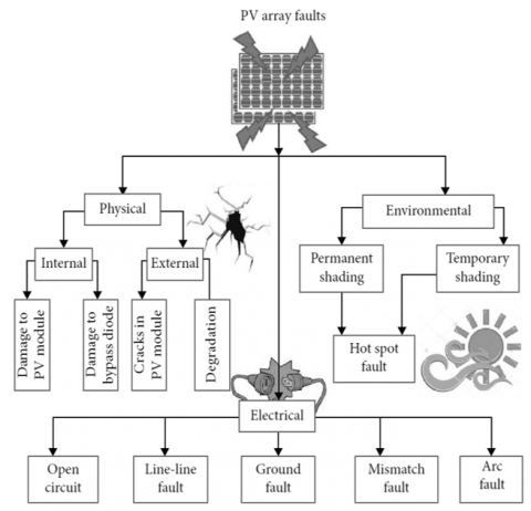
The rapid proliferation of grid-integrated renewable energy sources has led to the evolution of hybrid grids. However, the inconsistent characteristics of renewable energy power generation have resulted in challenges associated with power quality (PQ), system reliability, and stability, adversely impacting the operation of protective relays in real-time. Furthermore, high penetration of renewable energy sources into the utility grid could be achieved by employing multi-tapped transmission lines, particularly for the integration of wind and solar powers [3]. Such a development has posed substantial challenges for power system engineers in the design of suitable protection schemes. Different faults and incidents occurring on the power system network can engender problems relating to power quality, power system protection, and power network stability. The significance and severity of power system faults vary corresponding to the frequency of occurrence and magnitude of power flow in the network, as illustrated in Figure 1.

The penetration of renewable energy (RE) into utility networks has been increasing steadily, bringing into focus issues concerning energy security, equipment protection, grid security, power reliability, and power quality. The integration of RE near load centres has further exacerbated problems of false and delayed tripping within the protection system, primarily due to the uncertain and variable nature of RE generation. RE sources are known to cause considerable voltage transients and high current variations during outages and synchronization with the grid.

Short-circuiting of the modules composing a panel can lead to internal disruptions, resulting in decreased current and voltage readings, thereby reducing the total power output. This reduction can also be triggered by naturally existing external elements that diminish the amount of sunlight (irradiance) impinging on the surface of the solar panels, leading to dips in current and voltage readings and subsequently affecting the overall power output. A critical issue arises when changes in readings induced by internal defects are frequently conflated with those caused by external disturbances. It is crucial to address only the internal issues; the external disturbances, which could be as benign as a passing cloud, can often be overlooked.

The primary objective of this work is to isolate the internal (Line-to-Line or LL) faults that may be present within a panel and dismiss the decrease in power output triggered by external (shading) disturbances. This focus on internal faults allows for a more precise understanding and troubleshooting of issues that directly impact the efficiency and functionality of the solar panels.

1.png

Figure 1. Fault types in Solar panels

1.1 Implications of faults in solar panels

Faults within solar panels typically result in a reduction of maximum power generation. Instead of identifying the Global Maximum Power Point (GMPP), only the Local Maximum Power Point (LMPP) is detected, thereby diminishing the efficiency of the entire solar PV system [4]. Herein, Ipv and Vpv represent the PV array current measurement and voltage measurement, respectively, while Ia, Ib, and Ic denote current measurements of Phase_A, Phase_B, and Phase_C, respectively. Similarly, Va, Vb, and Vc correspond to voltage measurements of phases A, B, and C, respectively. These complexities highlight the necessity for swift fault detection and classification by PV installers or consumers to facilitate effective rectification.

In light of such challenges, a range of contemporary methods, including neural networks, fuzzy logic, and machine learning algorithms, has been successfully employed in the literature and has gained increasing popularity in the research field. Furthermore, various strategies, such as Particle Swarm Optimization (PSO), Ant Colony Optimization (ACO), Genetic algorithms, and advanced neuro-fuzzy methods, have been proposed and examined for monitoring the maximum power point under partially shaded conditions. These advanced methodologies aim to enhance the reliability and efficiency of solar PV systems by providing more accurate and timely fault detection and classification.

3.1 Deep sequential model

A deep sequential model, also known as a deep sequential neural network, is a type of artificial neural network that is designed to process data in a sequential or temporal manner. These models are commonly used for tasks involving sequences of data, such as time series analysis, natural language processing, speech recognition, and more. Deep sequential models are capable of learning complex patterns and dependencies within sequential data, which makes them suitable for a wide range of applications.

Key components and characteristics of deep sequential models include:

Sequential Processing: Deep sequential models process input data one step at a time, maintaining a sense of order or sequence. This is in contrast to feedforward neural networks, which take static inputs and produce static outputs.

Deep Architecture: Deep sequential models have multiple layers of processing units (neurons or cells) stacked on top of each other. These layers can be recurrent, convolutional, or a combination of both, depending on the specific architecture.

Recurrent Layers: Recurrent neural networks (RNNs) are a common choice for modeling sequential data. RNNs have connections that loop back on themselves, allowing them to maintain an internal state and capture dependencies over time.

Long Short-Term Memory (LSTM) and Gated Recurrent Unit (GRU): These are specialized recurrent layers that are designed to address the vanishing gradient problem in traditional RNNs. LSTMs and GRUs can capture long-term dependencies in data.

Convolutional Layers: In some cases, deep sequential models may also include convolutional layers, which are well-suited for tasks involving sequences with spatial components, such as image sequences or sensor data.

Variable-Length Inputs: Deep sequential models can handle input sequences of variable length. This flexibility is important for many real-world applications where the length of the sequence may vary.

Training: Training deep sequential models typically involves backpropagation through time (BPTT) for RNNs, which is a variant of the standard backpropagation algorithm. Training deep sequential models can be computationally intensive and may require careful initialization and regularization techniques.

Deep sequential models have been successfully applied to a wide range of tasks, including natural language understanding and generation, speech recognition, machine translation, sentiment analysis, video analysis, and more.

Common deep sequential model architectures include:

Recurrent Neural Networks (RNNs): Basic RNNs are the simplest form of deep sequential models. However, they have limitations in capturing long-range dependencies.

Gated Recurrent Unit (GRU) Networks: GRUs are another variant of RNNs, which are computationally more efficient than LSTMs while still being able to capture long-term dependencies as shown in Figure 2.

2.png

Figure 2. Gated Recurrent Unit (GRU)

Transformer-Based Models: Transformers have gained popularity for natural language processing tasks and sequence-to-sequence tasks. They use self-attention mechanisms to capture dependencies in input sequences.

Deep sequential models have significantly advanced the state of the art in many areas of artificial intelligence and machine learning. They are a fundamental tool for modeling and making predictions on sequential data. Deep sequential models are implemented when the input and output are both data sequences as shown in Figure 3. The points of data can be arranged into sequences so that significant data about observation performed at subsequently points in the collection may be deduced from measurements performed at a single instance in the sequence. The sequence learning issue can occur when a parameter is a sequence and an output is a single data point, as in the instances of video action identification, sentiment classification, and stock price predictions.

For sequence data, managing ongoing supervised learning processes is necessary [11]. The combined length of the sequences used for input and output may vary and may appear the same or different in instances where both the input and the result are sequences, such as recognition of speech, natural language understanding, and sequence DNA analysis. Neural networks based on deep learning have mostly been applicable to speech recognition, natural language processing, and picture analysis since they demonstrate the capacity to capture extremely complex input and output mapping [12]. This approach ultimately led to the development of multiple deep-learning time series forecasting structures that exceed conventional methods in terms of precision and efficacy.

3.png

Figure 3. Deep sequential model

3.1.1 Long short-term memory networks

Recurrent neural networks serve in the analysis of input neural network categories in sequence. Because of these hidden states, previously predicted amounts can be used as inputs as shown in Figure 4.

4.png

Figure 4. Recurrent neural networks model

An RNN comprising input, output, and a hidden layer make up a multilayer perceptron [13]. The n layers that make up a multi-layered perceptron are established by the particular order in which they are generated. The Keras software platform was employed to create the deep learning algorithm. As data shows up, is stored by the algorithm, and becomes available points, a structure must be maintained. An input gate, a memory gate, and an output gate were the three gates that LSTMs utilize. Each of the three of these gates, that compose the vast majority of the LSTM model shown in Figure 5, are in the position of regulating the monitoring of everything. Eq. 1 indicates that the recollecting component of the gate utilizes a combination of the previously concealed state and the data item being processed by the sequencing gate to identify which components of the LSTM should now be removed [14].

5.png

Figure 5. Long short-term memory model

Equation is the input component of the computational Eq. 2 with the gate.

$F(t)=\sigma\left(W_f\left[h_{t-1}, X_t\right]+b_f\right)$           (1)

$I(t)=\sigma\left(W_f\left[h_{t-1}, X_t\right]+b_i\right)$      (2)

$f(x)=\frac{1}{1+e^{a x t}}$      (3)

$\tanh (x)=\frac{2}{1+e-2^x}-1$     (4)

The newly developed concealed state includes to be generated through the output gates. The most recently updated input data, the least current concealed state, and the most current real state of cells were all taken into consideration when choosing the option that was made. The remember gate, input gate, and output gate weight values were Wf, Wi, and Wo, correspondingly. The response to Eq. 4 indicates that the formula operator sigmoid used data from both the most current input and the previously provided hidden layer input [15]. The (tanh) function has been utilized to communicate data regarding the parameters connected to the input to the gate, the current source, and its previously concealed state. Whereas the range of a sigmoid () function's value is 0 to 1, those of the tanh function is -1 to 1.

3.1.2 Multilayer perceptron

An artificial neural network with multiple layers of connected neurons or nodes is referred to as a feedforward neural network, or multilayer perceptron (MLP) as shown in Figure 6. Information passes from the input layer to the final layer of output through the hidden layers.

Machine learning tasks including pattern recognition, regression, and classification belong to several applications for MLPs.

Key characteristics of a Multilayer Perceptron as shown in Figure 6:

Input Layer: The nodes in this layer represent in all the variables that have been entered. The number of nodes in this layer is decided by the dimensionality of the input data, each node indicating a feature.

Hidden Layers: There could be one or more hidden layers in between the input and output layers. Nodes in these categories conduct out computations and transform the input data into a format appropriate for the output. Hyper parameters that can be modified are the amount of nodes in each layer and the number of hidden stages.

Output Layer: The algorithm's final predictions or outputs are produced by the output layer. The type of analysis being performed (e.g., regression, multi-class classification, binary classification) affects how many nodes belong to this layer.

6.png

Figure 6. Multi-layer perceptron

7.png

Figure 7. The progression of the process

Another type of artificial neural network that is frequently used for image and video recognition applications is a convolutional neural network (CNN). They were designed to process input data having a structure resembling a grid, like an image.

An MLP can process the contextual data, such as maintenance logs or historical operating conditions, while an LSTM can capture temporal dependencies in sensor data. The combined model can predict equipment failures more accurately.

Hybrid models that combine Multilayer Perceptrons (MLPs) and Long Short-Term Memory (LSTM) networks can be powerful tools in machine learning, especially when dealing with complex data that includes both structured and sequential components. The progession of the process is as shown in Figure 7.

5.1 Performance metrics

It is essential to choose the appropriate performance criteria for the purpose of assessing machine learning and deep learning algorithms successfully. They mainly used the performance statistics of recall (R), accuracy (A), precision (P), and F1-score (F1) to satisfy the objective of this research.

precision $=\frac{\text { True positive }(T p)}{\text { True positive }(T p)+\text { False positive }(F p)}$     (5)

Recall $=\frac{\text { True positive }(T p)}{\text { True positive }(T p)+\text { False Negative }(F n)}$     (6)

Accuracy $=\frac{T p+T N}{T p+T N+F P+F N}$     (7)

F1score $=2 * \frac{\text { Recall } * \text { precision }}{\text { Recall }+ \text { precision }}$    (8)

Table 1 presents the accuracy, precision, recall, and F1 score results for the Random Forest classifier, K-nearest neighbor, SVM classifier, ensemble learning, and proposed model results. The technique to evaluate a machine learning model's performance based on multiple subsets of the training data is known as cross-validation. The standard deviation of the performance metrics across these subsets can give you an idea of how stable the model's performance is. A lower standard deviation generally indicates more consistent and stable performance.

Table 1. Assessment of model output parameters

The standard deviation of a machine learning model's performance metric is a measure of the model's consistency. A low standard deviation indicates stable and predictable performance, while a high standard deviation suggests less stable and inconsistent performance. When comparing different models or evaluating the same model under various conditions, it's often preferable to choose the model with lower standard deviation, as it is more likely to generalize well to new, unseen data. However, it's crucial to consider other factors and conduct a comprehensive evaluation of model performance, as standard deviation alone may not capture all aspects of a model's behavior.

Our proposed model got very good standard deviation value 0.99942, which shows the stability of the model.

The faults were manually introduced in the middle of the experiments. The readings at high frequencies are erratic. Between the scenarios and throughout them, there are disruptions. Temperature and insolation change throughout the trials and between them. The issue is to find and diagnose the defects before they result in such a complete failure because in critical fault scenarios, the operation is halted and the system may shut down. Furthermore, MPPT/ IPPT modes impair the ability to identify low-magnitude faults. The results of the prediction are shown in Figures 7 and 8.

Figure 9 shows the Confusion matrix of the model, is a valuable for understanding a model's strengths and weaknesses, particularly in situations where one type of error (false positives or false negatives) is more costly or critical than the other. Analyzing the confusion matrix helps you fine-tune the proposed machine-learning models and make informed decisions about model improvements or adjustments.

8.png

Figure 8. Plotting the reduced dimensionality data with the corresponding fault label

9.png

Figure 9. Confusion matrix of prediction