Inas A. Al-Tahar*![]() | Assad Al-Shueli
| Assad Al-Shueli![]()
© 2023 IIETA. This article is published by IIETA and is licensed under the CC BY 4.0 license (http://creativecommons.org/licenses/by/4.0/).
OPEN ACCESS
Frequency estimation of sinusoidal signals is a critical task in various signal processing applications, including control systems, monitoring, radio broadcasts, and more. The Fast Fourier Transform (FFT) is a widely employed technique for signal analysis; however, it suffers from spectral leakage issues. To mitigate this problem, windowing functions are utilized, aiming to enhance frequency estimation accuracy through the combination of an optimal window and a precise frequency correction formula. In this study, a novel frequency estimation algorithm based on a three-point spectral interpolation method is proposed and compared with the Jacobsen algorithm. Simulation results demonstrate that the proposed algorithm exhibits superior performance in terms of frequency estimation errors. Specifically, the maximum frequency estimation error for the proposed algorithm, when using the Nuttall window, was found to be 0.001, representing a 29-fold reduction compared to the error of 0.029 for the Jacobsen algorithm. This improvement highlights the effectiveness of the proposed interpolation-based algorithm for accurate frequency estimation in signal processing applications.
interpolation methods, frequency estimation, frequency-domain analysis, FFT, FPGA, Jacobsen algorithm
Estimating the frequency of a sinusoidal signal is an important task in signal processing in many applications such as control, monitoring, radio broadcasts and others. On the other hand, the signal processing performance of the spectral analyses of the sinusoidal waveforms may be usefully utilized in the field of the measurements on the power systems [1]. The Fast Fourier Transform (FFT) is one of the most common procedures used in digital signal processing [2]. The discretization of the signal leads to the fact that the amplitude spectrum of the signal is infinitely repeated on the frequency axis with a period equal to =1/Td. FFT is an algorithm that computes the Discrete Fourier Transform (DFT) of a sequence. DFT is a discrete frequency spectrum much like a time domain signal is formed by an ADC. The result of the DFT is similar to viewing a continuous windowed spectrum through a picket fence with slots in the intervals corresponding to the frequency slots.
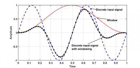
Kotelnikov's theorem states that a signal can be completely reconstructed from discrete, equally spaced samples if the sampling rate is at least twice the highest frequency of that signal. If the signal is not with an integer number of periods within the sampling window, then there will be discontinuities at the boundaries of this window, which result in additional spectral components in the frequency domain, known as spectral leakage or spectrum spreading. To minimize spectral leakage, the data samples at the beginning and end of the signal are smoothed by reducing them to zero. The smoothing of the time sequence consists in multiplying all signal samples by the weight coefficients of a special function called the "window" as shown in Figure 1. A large number of windows have been developed that differ in terms of resolution, degree of smoothing, influence on the signal-to-noise ratio, etc.
High-performance computing algorithms are available to perform digital signals DFT [3]. The spectral leakage problem occurs when the number of sample signal periods is not integer number, when the sampling process is not synchronized with the main component of the test signal [4-7]. In this paper, simple interpolation formulas with a Nuttall window were used to reduce the spectral leakage effect for precise frequency detection. This approach has high accuracy in frequency estimation. Many frequency assessment studies have been conducted [8-13]. The 4-point model-normalized algorithm, bounded by least squares, was poorly evaluated [8]. Integrated treatment approach was studied to reduce spectrum leakage [9]. Kaiser-based window algorithm was proposed to minimize the spectral leakage effect [10]. Luo et al. [11] uses zero completion in window algorithms. The work of the iterative algorithm is suggested [12, 13]. In this algorithm A&M-estimation is used to improve the evaluation performance. In 2007, Jacobsen et al. [14] proposed a trispectral correction algorithm, in which the normalized correction frequency expression suitable is:
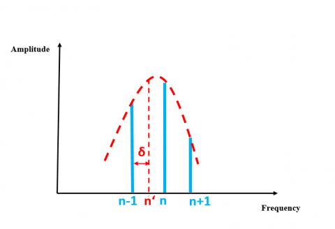
$\delta=\frac{\left|U n_{+1}-U n_{-1} \;\right|}{\left|4 * U n-2 * U n_{+1}-2 * U n_{-1}\; \right|}$ (1)
where, $U n, U n_{+1}, U n_{-1}$ and are shown in Figure 2a, $\delta$ is the frequency deviation from true frequency is determined by the mutual position of the line of the spectrum of maximum amplitude and the second line of the spectrum of maximum amplitude (see Figure 2a and Figure 2b).
An uncomplicated algorithm has been suggested in this paper to canceling the spectral leakage used multiplying the respective signal by a time window, equation for correction frequency using linear interpolation shown in Eq. (4) were able to additionally enhance the accuracy of the estimation. In comparison to existing algorithms, the suggested algorithm presents a lower computational complexity and a better performance of estimation.
Figure 1. Effect the window on the signal
The rest of this paper is as follows: In the second section the proposed algorithm described. In the third section the results and discussion are described, Conclusions presented in the last section.
Figure 2a. Spectrum DFT (signal frequency is between n and n+1)
Figure 2b. Spectrum DFT (signal frequency is between n and n-1)
Figure 2c. Spectrum DFT (signal frequency is in n exactly)
The general procedure of the interpolation estimator is shown in Figure 3. A sampled signal's time domain form can be written as [15].
$X(n)=A \sin (2 \pi F c \ n / F s +ȹ)$ (2)
where, Fs is the sampling frequency, n=0, 1, 2..., N - 1, A is the amplitude, ȹ is the starting phase angle, and Fc is the fundamental frequency. The total number of sampling sites is N. Using a window function, w(n), and continuous Fourier transform, it is possible to produce discrete estimate sequences of the sampled signal in the frequency domain, X(f).
$\mathrm{X}(\mathrm{f})=\sum_{n=-\infty}^{\infty} x(n) w(n) e^{-j 2 \pi f n}$ (3)
The algorithm for determining the frequency from the spectrum with an estimate of the methodological error of the simulation can be represented in the form of steps:
1. Select range of signal frequencies Fc, Sample size (N), sampling frequency Fs, and type of window.
2. Apply windowing function on the resulting array.
3. Compute FFT.
4. Determine the number of the component whose amplitude is maximum in the complex spectrum FFT.
5. Find the spectral lines left and right closest to the maximum component.
6. By propose formula calculate (delta δ) the correction formula of frequency offset between n and index n' corresponding to the maximum amplitude in the spectrum. As shown in Figure 2a.
$\Delta 1=\frac{U n}{U n_{-1}}$ (4)
$\Delta 2=\frac{U n}{U n_{+1}}$ (5)
$\delta=\frac{(\Delta 2 / \Delta 1)-1}{(\Delta 2 / \Delta 1)+1}$ (6)
7. The signal frequency calculated:
Fest $=(\mathrm{n}+\delta) * \frac{\mathrm{Fs}}{\mathrm{N}}$ (7)
8. Estimate of the error of the frequency estimation by:
Erest $=(($ Fest $-\mathrm{Fc}) / \mathrm{Fc})$ (8)
Figure 3. Procedure of the general interpolation method
This section presents the results of modeling the algorithm proposed above. The considered parameters are closely related to the signal in the Eq. (3). Let's consider an example of monitoring the frequency of a power supply network of 50 Hz, with a 1 Hz deviation frequency. A suitable frequency resolution value must be taken into account. This value should be small enough so that all of the signal components seem as certain spectral lines that are related to relative maximum points after the operation of the FFT. In order to do this, it suffices to take under consideration a suitable number of the samples, based on Δf= Fs/N=1/NΔt. Fs and samples values have been chosen as: Fs= 256 Hz, and N=256 samples.
An analytical comparison was made between the proposed algorithm and Jacobsen’s algorithm shown in Figure 4 when Nuttall window is used. The value of the maximum systematic error in the Jacobsen algorithm was 0.029, while it was in the proposed algorithm 0.001 when sample size is 256, which means that the number of improvement times is 29. The simulation showed that the abrupt discontinuity in Figures 4 especially when Fc=50.5 Hz is due to a change in the structure of an odd number of components taken into account at the maximum of the energy spectrum with two components, as shown in Figure 2.
Depending on the ratio of the frequency of the fundamental signal to the sampling frequency, the following spectrum structures can be distinguished:
1. Symmetry with respect to the central component close to the desired signal frequency (Figure 2a).
2. Symmetry with respect to two neighboring components, between which the desired signal frequency is located (Figure 2 b, c).
For the purpose of verifying the effectiveness of the suggested windows and the algorithms of the interpolation, second simulations were performed. The analysis results shown in Figure 5, in which the error curves of frequency estimation measurements versus the ratio (Fc/Fs=4) are shown, for different size of samples. In particular, the maximum error curves of the frequency measurements for N= (32-8129) have been respectively reported.
Moreover, an FPGA implementation of real-time interpolation is presented in Figure 6. The interpolator's approach is based on a one-dimensional Fast Fourier Transform (FFT).
This requires the use of MATLAB with Xilinx ISE 14.4. You must be familiar with the MATLAB program and Verilog high-fidelity modeling languages. One needs to be accustomed to the Discrete Fourier Transformation in order to understand the design. Spartan 3E-100 (xc3s100e) and a computer running Fpga programmer, Function Generator, Diligent, and Oscilloscope are needed for the project's physical needs.
Figure 4. Relative frequency estimation error for Nuttall window
Table 1. Relative maximum frequency estimation error
|
Size of sample (N) |
Maximum frequency estimation error |
|
|
Jacobsen algorithm |
Proposed algorithm |
|
|
32 |
0.17 |
0.003 |
|
256 |
0.02 |
0.0008 |
|
8192 |
0.0007 |
0.00002 |
Figure 5. Relative maximum frequency estimation error for Nuttall window
Figure 6 depicts the simulation and implementation process. The in and out pin blocks define the hardware's boundaries after several methods have been used to select the best design. With the help of the implementation on the hardware and Xilinx software such as nets list, bits flow, and time analysis, resource usage has been determined.
The majority of recent studies [16-20] aim to decrease the set time deviation in order to lower the system size. However, on ASIC FPGA systems, reducing hardware size alone does not entirely contribute to cost savings in the physical design. Additionally, a smaller method may result in a longer word length size, which would increase unnecessary hardware and dramatically lower the SNR.
The FPGA's parallelism functionality is used in the current work to reduce computing time without compromising system complexity. Due to the FPGA resource's plenty of switches and millions of transistors, the current system was developed using a parallel approach design using a low-power algorithm and hardware structure.
With the help of the Xilinx platform generator platform Version 14.2, equipment on the Spartan 3E-100-CP132 is simulated. This application installs the FPGA block set required for embedded systems in the Matlab and Simulink library browsers.
Moreover, an FPGA implementation of real-time interpolation is presented in Figure 7. The interpolator's approach is based on a one-dimensional Fast Fourier Transform (FFT).
This requires the use of MATLAB with Xilinx ISE 14.4. You must be familiar with the MATLAB program and Verilog high-fidelity modeling languages.
One needs to be accustomed to the Discrete Fourier Transformation in order to understand the design. Spartan 3E-100 (xc3s100e) and a computer running FPGA programmer, Function Generator, Diligent, and Oscilloscope are needed for the project's physical needs.
Figure 6. For an FPGA board, the design algorithm produces synthesizable RTL
Figure 7. The algorithm implementation on FPGA
The implementation was synthesized on an FPGA board, and the process calculation has been optimized using a parallel technique to decrease the FPGA's area and power requirements as shown in Figure 7.
Additionally, the implementation constraints of the Frequency Estimation Technique Utilizing a Three-Point Spectrum Interpolation may result in computing time savings, which is an important consideration in design approach. Because the output of these methods is mostly based on frequency domain rather than the time domain, stability is the key problem in their design.
In this paper, a new and accurate estimator algorithm for the electrical network frequency of real sinusoids is proposed using the three-point interpolation of DFT samples. In this algorithm, the electrical signal is multiplied by a time window to reduce the spectral leakage arising as a result of the fast Fourier transform process. Three windows are used and the experimental results of these windows are compared. The Nuttall window outperformed the other windows in the evaluation, as it gave the lowest error rate, from the analysis of this study and Table 1, the remarks below are noteworthy.
[1] Eslami, A., Negnevitsky, M., Franklin, E., Lyden, S. (2022). Review of AI applications in harmonic analysis in power systems. Renewable and Sustainable Energy Reviews, 154: 111897. https://doi.org/10.1016/j.rser.2021.111897
[2] Rajaby, E., Sayedi, S.M. (2022). A structured review of sparse fast Fourier transform algorithms. Digital Signal Processing, 103403. https://doi.org/10.1016/j.dsp.2022.103403
[3] Joseph, C., Prakash, S.S. (2022). Design of Efficient Pruning Architecture for FFT Algorithm. In 2022 First International Conference on Electrical, Electronics, Information and Communication Technologies (ICEEICT) Trichy, India, pp. 1-6. https://doi.org/10.1109/ICEEICT53079.2022.9768412
[4] Jiao, L., Du, Y. (2022). An approach for electrical harmonic analysis based on interpolation DFT. Archives of Electrical Engineering, 71(2): 445-454. https://doi.org/10.24425/aee.2022.140721
[5] Ma, X., Yang, Q., Chen, C., Luo, H., Zheng, D. (2020). Harmonic and interharmonic analysis of mixed dense frequency signals. IEEE Transactions on Industrial Electronics, 68(10): 10142-10153. https://doi.org/10.1109/TIE.2020.3026288
[6] Wang, X., Szydlowski, M., Yuan, J., Schwingshackl, C. (2022). A multi-step interpolated-FFT procedure for full-field nonlinear modal testing of turbomachinery components. Mechanical Systems and Signal Processing, 169: 108771. https://doi.org/10.1016/j.ymssp.2021.108771
[7] Jwo, D.J., Wu, I.H., Chang, Y. (2019). Windowing design and performance assessment for mitigation of spectrum leakage. In E3S Web of Conferences, 94: 03001. https://doi.org/10.24425/aee.2022.140721
[8] Li, Z., Xia, Y., Wang, Q., Pei, W., Hao, J. (2019). A novel four-point model based unit-norm constrained least squares method for single-tone frequency estimation. IEICE Transactions on Fundamentals of Electronics, Communications and Computer Sciences, 102(2): 404-414. https://doi.org/10.1587/TRANSFUN.E102.A.404
[9] Wang, Q., Yan, X., Qin, K. (2014). Parameters estimation algorithm for the exponential signal by the interpolated all-phase DFT approach. In 2014 11th International Computer Conference on Wavelet Actiev Media Technology and Information Processing (ICCWAMTIP), pp. 37-41. https://doi.org/10.1109/ICCWAMTIP.2014.7073356
[10] Bai, G., Cheng, Y., Tang, W., Li, S., Lu, X. (2019). Accurate frequency estimation of a real sinusoid by three new interpolators. IEEE Access, 7(1): 91696-91702. https://doi.org/10.1109/ACCESS.2019.2927287
[11] Luo, J., Xie, Z., Xie, M. (2016). Interpolated DFT algorithms with zero padding for classic windows. Mechanical Systems and Signal Processing, 70(1): 1011-1025. https://doi.org/10.1016/j.ymssp.2015.09.045
[12] Ye, S., Sun, J., Aboutanios, E. (2017). On the estimation of the parameters of a real sinusoid in noise. IEEE Signal Processing Letters, 24(5): 638-642. https://doi.org/10.1109/LSP.2017.2684223
[13] Ye, S., Sun, J., Aboutanios, E. (2018). Corrections to “On the Estimation of the Parameters of a Real Sinusoid in Noise”. IEEE Signal Processing Letters, 25(7): 1115-1115. https://doi.org/10.1109/LSP.2018.2846138
[14] Jacobsen, E., Kootsookos, P. (2007). Fast, accurate frequency estimators [DSP Tips & Tricks]. IEEE Signal Processing Magazine, 24(3): 123-125. https://doi.org/10.1109/MSP.2007.361611
[15] Jin, T., Chen, Y., Flesch, R.C. (2017). A novel power harmonic analysis method based on Nuttall-Kaiser combination window double spectrum interpolated FFT algorithm. Journal of Electrical Engineering, 68(6): 435-443. https://doi.org/10.1515/jee-2017-0078
[16] Kumar P. (2012). Generating, optimising and verifying HDL code with MATLAB and simulink. The MathWorks, Inc. https://www.mathworks.com/content/dam/mathworks/mathworks-dot-com/solutions/automotive/files/in-expo-2013/generating-optimizing-and-verifying-hdl-code-with-matlab-and-simulink.pdf.
[17] Guan. X, Fei. Y, Lin. H, (2012). Hierarchical design of an application-specific instruction set processor for high-throughput and scalable FFT processing, IEEE Transactions on Very Large Scale Integration (VLSI) Systems, 20(3): 551-563. https://doi.org/10.1109/TVLSI.2011.2105512
[18] Chang W.H., Nguyen T. (2007). Integer FFT with optimized coefficient sets. P 2007 IEEE International Conference on Acoustics, Speech and Signal Processing - ICASSP '07, Honolulu, HI, USA, pp. II-109-II-112. https://doi.org/10.1109/ICASSP.2007.366184
[19] Ghouwayel. A.A., Louet. Y. (2009). FPGA implementation of a re-configurable FFT for multi-standard systems in software radio context. 2009 Digest of Technical Papers International Conference on Consumer Electronics, Las Vegas, NV, USA, 2009, pp. 1-2. https://doi.org/10.1109/ICCE.2009.5012170
[20] Chang, W., Nguyen T.Q. (2008). On the fixed-point accuracy analysis of FFT algorithms. IEEE Transactions on Signal Processing, 56(10): 4673-4682. https://doi.org/10.1109/TSP.2008.924637