Paul Menounga Mbilong* | Asmae Berhich | Imane Jebli | Asmae El Kassiri | Fatima-Zahra Belouadha
© 2021 IIETA. This article is published by IIETA and is licensed under the CC BY 4.0 license (http://creativecommons.org/licenses/by/4.0/).
OPEN ACCESS
Coronavirus 2019 (COVID-19) has reached the stage of an international epidemic with a major socioeconomic negative impact. Considering the weakness of the healthy structure and the limited availability of test kits, particularly in emerging countries, predicting the spread of COVID-19 is expected to help decision-makers to improve health management and contribute to alleviating the related risks. In this article, we studied the effectiveness of machine learning techniques using Morocco as a case-study. We studied the performance of six multi-step models derived from both Machine Learning and Deep Learning regards multiple scenarios by combining different time lags and three COVID-19 datasets(periods): confinement, deconfinement, and hybrid datasets. The results prove the efficiency of Deep Learning models and identify the best combinations of these models and the time lags enabling good predictions of new cases. The results also show that the prediction of the spread of COVID-19 is a context sensitive problem.
deep learning, machine learning, COVID spread prediction
Over the past 20 years, advanced data technologies and Artificial Intelligence (AI), especially Machine Learning (ML) and Deep Learning (DL), have transformed the medicine and epidemiology field. In fact, ML is used to study the risk stratification for specific infections, identify the relative contribution of specific risk factors to overall risk, understand pathogen-host interactions, and predict the emergence and spread of infectious diseases [1].
Coronavirus 2019 (COVID-19) is has become, according to the World Health Organization, an international epidemic having caused 21 294 845 cases, and 680 894 deaths on August 17, 2020 [2]. It is considered as the most crucial global health crisis of the century that has an emerging wide socio-economic and health impacts, and is a great challenge that the governments face. Given the high value of R0 index against the fragility of the health structure and the scarcity of test kits, especially in developing countries, forecasting the spread of COVID-19 should help decision-makers to better manage the crisis situation (health protocols, resource sharing, distance education, distance work, required masks and test kits, confinement/deconfinement…), and contribute to mitigate the related risks on socio-economic and health fields.
In this context, recent research work has studied how to help governments using ML and DL technologies to manage the current pandemic situation. Different learning models have been separately experimented on different countries, and have led to different accuracies that should be improved. Given the specificity of the COVID-19 context and the fact that COVID-19 spread forecasting is a time-series problem, we think that it would remain interesting to experiment different learning models applied to a same context using multi-step models and assessing different time lags (fixed amounts of passing time). This would help to identify the best models for COVID-19 spread forecasting and the best time lags to be considered for these models in order to ensure good predictions and accuracies.
In this perspective, after selecting six different regression techniques: Linear Regression (LR) and Random Forest (RF) that are ML techniques, and Multilayer Perceptron (MLP), Long Short-Term Memory (LSTM), Gated Recurrent Units (GRU), and Convolutional Neural Network (CNN) that rather fit to DL techniques, we analyzed their performance while using different time lags and experimenting with three Morocco’s datasets: confinement, deconfinement and hybrid datasets. The selected models were trained to predict new cases that will be reported during a future 7 days from previous data (new cases) reported during different time lags (fixed amounts of passing time).
The remainder of this paper is organized in five sections. Section 1 is devoted to related work. Section 2 presents the selected models used in our study. Section 3 describes the artifacts of the performed learning processes. Section 4 presents and discusses the obtained results. Finally, Section 5 summarizes the conclusions and perspectives of this work.
For the purpose of predicting epidemic outbreaks (e.g., Ebola, Cholera, swine fever, H1N1 influenza, dengue fever, and Zika), scientists have usually used the Susceptible-Infected-Resistant (SIR)-based models. However, the results obtained while using these models in the context of COVID-19 have showed some degree of uncertainties [3]. This virus has demonstrated an irregularity in its spread that encourages the emergence of advanced epidemiological models [3, 4]. In this perspective, ML that has gained attention for building outbreak prediction models [3] like random forest for swine fever prediction [5, 6], neural network for H1N1 flu, dengue fever, and Oyster norovirus [7-9], classification and regression tree (CART) for Dengue [10], has also been adopted for predicting COVID-19 outbreaks.
Adaptive network-based fuzzy inference system (ANFIS), multi-layered perceptron-imperialist competitive algorithm (MLP-ICA), and logistic, linear, logarithmic, quadratic, cubic, compound, power and exponential regression have been used by Ardabili et al. [11] to investigate their generalization ability for predicting the virus outbreaks in different countries. MLP and ANFIS showed promising results. However, they should be experimented on different countries with different contexts (different social culture, different health structures…) to confirm these findings.
The Kermack-Mckendrick SIR and Prophet models have been applied by Ndiaye et al. [12] to predict the inflection point and the possible ending time. It has been expected that the pandemic in some countries (like China) will end soon within few weeks, while the hit of anti-pandemic will be no later than the end of April for most part of countries in the world (Italy, Iran and Senegal).
Six regression-based models (quadratic, third degree, fourth degree, fifth degree, sixth degree and exponential polynomial have been used by Yadav et al. [13] to predict the number of Indian patients suffering from the COVID-19. The authors think that the sixth-degree polynomial regression model will help doctors and the government to prepare their plans for the next 7 days. However, they have focused on regression models only without comparing their relevance to that of DL models that are actually considered as promising models in Artificial Intelligence field.
Two hybrid models (ANFIS and MLP-ICA) have been used by Pinter et al. [3] to predict new cases and mortality rate in Hungary. The authors concluded that by late May, the outbreak and the total morality would drop substantially while the best RMSE metric for the MLP-ICA model was 167.88. However, they think that advancing deep learning models are strongly encouraged for comparative studies on various ML models for individual countries.
A variant of the SEIR (Susceptible - Exposed - Infectious - Recovered) model has been used by Zou et al. [14] to predict confirmed and fatality cases in the United States by taking into account the untested/unreported ones, and facilitate the decision-making process. The proposed model provides both short-term (daily ahead) and long-term projections. The prediction results suggest that the numbers of confirmed cases and death will keep increasing rapidly within one month. However, the authors note that their model does not take into consideration how the reopening orders affect the virus spread and the contact rate.
Random Forest and Kalman filter have been used to predict the rate of propagation, mortality and active cases in India [15]. However, it has been noted that the proposed model shows large mean average error for long-term prediction and that it is good for short-term prediction (daily and weekly).
The behavior of the Random Forest (RF) machine learning algorithm has been again studied by Yeşilkanat et al. [16] this to estimate the future number of COVID-19 cases over 190 countries in the world and it is mapped to the true results of the confirmed cases. however, the author did not provide information on the earlier number of days used for predicting upcoming days.
A nested sequence prediction using a Long Short-Term Memory (LSTM) model has been used by Bouhamed et al. [17] to monitor infection and recovering processes in different countries. The author thinks that the results are very encouraging with a R2 score equal to 0.99. However, the curve drawing the prevision of confirmed case and the real ones for France in 6 days shows deviations that are close to about 5000 cases.
Chimmula et al. [18] have also used an LSTM model to predict for 2 successive days, the future COVID-19 in 2, 4, 6, 8, 10, 12 and 14 next days, and to compare the transmission rates in Canada with that of Italy and USA. In the Canadian dataset, the RMSE error was 34.83 with an accuracy of 93.4% in training set and 45.70 with an accuracy of 92.67% in test set. The obtained results showed that the stopping time of the virus outbreak would be around June 2020. However, these projections did not take place.
For deep learning prediction, it is sometimes interesting to predict several future values of a variable based on several past values. The models elaborated with this objective are grouped under the term sequence to sequence (seq2seq). These models take m past values (m lags) and try to predict n future values (n steps). Liu et al. [19] have e.g., proposed a seq2seq model that can give a reliable alert 2 hours in advance before air pollution suddenly strikes. Hao et al. [20] have used a LSTM model that predicts the number of passengers expected at subway stations in the near future, has been proposed. The predictions are performed given the number of passengers who have boarded at each station during the last periods of time. In this paper, we think that predicting the propagation of Covid-19, should be performed for several coming days to give enough time to governments to make decisions, and should also be based on several past days since the incubation period for COVID-19 is on average 5-6 days, and can be up to 14 days. Thus, we experiment our models with different sequences to found the appropriate ones according to the epidemic context and the size of the available data. Increasing both the size of the time lags and the time step, should be in fact, done minutely, since it will decrease the number of sequences to be studied, and hence, the model’s performance due to the incapability of deep learning models to well learn from small datasets.
In summary, advanced researches exploring, especially the promising DL models for more accurate COVID-19 spread predictions, remain strongly encouraged.
ML is a branch of AI that is able to learn successfully complex patterns from observed data to make predictions about unobserved data [21]. However, ML techniques are more suitable to linear problems but they present limitations in dealing with unstructured or complex problems. Besides, DL that is a class of ML algorithms, uses neural networks to detect complex and inherent relationships in data. DL techniques perform well with both linear and nonlinear data. Nevertheless, they need sufficient representative input data in a way that makes it possible to capture the underlying structure and to generalize to new observations [22].
Given the strengths and weaknesses of both ML and DL techniques, we have selected six different regression techniques related to the most powerful and popular categories to perform our study. Linear Regression (LR) and Random Forest (RF) that are ML techniques, and Multilayer Perceptron (MLP), Long Short-Term Memory (LSTM), Gated Recurrent Units (GRU), and Convolutional Neural Network (CNN) that rather fit to DL techniques.
LR enables evaluating the relative impact of a predictor variable x on a particular outcome y. It consists of finding the best-fitting straight line through the points obtained when the predictions of y are plotted as a function of x Figure 1, and it is more suitable to be used for data with linear relationship [23].
Figure 1. Linear regression technique
Figure 2. Random forest technique
RF helps generating different models in such a way that the combination of their results reduces the generalization error. It consists as shown in Figure 2, of building decisions trees by randomly selecting outcomes among the features for every decision tree, and then averaging these predicted outcomes [24]. Being an effective alternative to SVM [25], it is one of the most accurate learning algorithms even if it has been observed to overfit when there are regression tasks or noisy classification [26]. Note also that RF makes a wrong prediction only when more than half of the base classifiers are wrong.
MLP is an Artificial Neural Network (ANN) that is also a Feed-Forward Neural Network (FFNN) [27]. Being inspired by biological neural networks, ANNs are able to learn through experience. They are neural networks that could detect the patterns and relationships in data. As shown in Figure 3, an ANN is formed from a set of artificial neurons connected with weights and organized in layers [28]: Input layer, one or more hidden layers and output layer [22]. Input layer receives the input data. Hidden layer performs transformations. Each neuron uses activation function to transform weighted inputs (weighted sum) into one output. Output layer returns the output data (the predicted value in regression). Note that activation function introduces non-linearity to the network according to different computations as shown in Figure 3. Besides, in order to learn and perform accurate predictions, an ANN is trained in such way that the weights are optimized until the error in predictions is minimized. ANNs are suitable to find nonlinear relationships between outcome and predictor variables, and able to deal with noise and complex data. However, the behavior of an ANN depends of its architecture and the activation functions and the learning rule that it uses.
Besides, an ANN/FFNN network is an ANN network whereby information moves from input nodes to hidden layer and then output nodes. MLP fits to this category and is an advanced variation of ANNs that uses Backpropagation (BP). In other terms, it calculates weights using the propagation of the backward error gradient, and performs more phases in the learning cycle to train a multilayer network. Even if it seems to be more difficult to optimize, it still remains a simple network able to give better generalization and a powerful prediction thanks to its multilayer nature, nonlinear activation and BP learning.
Figure 3. Basic ANN and MLP technique
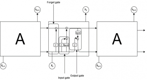
LSTM network [29] is an advanced variation of Recurrent Neural Networks (RNNs) that are able to remember what happened in the past in order to predict the future. They are multi-layer ANNs that are good for sequential data [30] since they bring neurons forming time sequence and benefit from extra memory to analyze input sequences [25] and hence, temporal behavior. Being an RNN network, an LSTM network Figure 4 is formed of different parts A, each transforming in a given step, an input xt into an output ht (information), which will be passed to the next step. Moreover, it benefits of a gated memory unit with three gates that enable remembering longer periods by memorizing network parameters for long durations. Each part A is composed out of four layers: a sigmoid layer combined with a pointwise multiplication operation to form an input gate, a sigmoid and a tanh layers combined with pointwise multiplication and addition operations to compose a forget gate, and finally, a sigmoid layer combined to the tanh function, and a pointwise multiplication operation to form an output gate. The three gates indeed allow the neural network to selectively remember and forget information in each step by selecting the appropriate ones and then adding them to the memory cells before finally deciding of what value it would be output. Note that LSTM was designed to avoid the RNN’s limitations, especially vanishing gradient problems. It can also adapt nonlinearities of input data [18], and is a powerful algorithm for implementing a sequential time-series model.
Figure 4. LSTM technique
GRU network is a simpler variation of LSTM neural networks that involves less parameters. As illustrated in Figure 5, it considers only two gates: an update gate z and a reset gate r. The update gate is used to determine how much of previous memory to keep around, whereas the reset gate is used to combine new input with previous value. It is worth mentioning that GRU network is faster to train and needs fewer data to generalize. It also has comparable performance to, or even may lead to better results than, LSTM network [31].
Figure 5. GRU technique
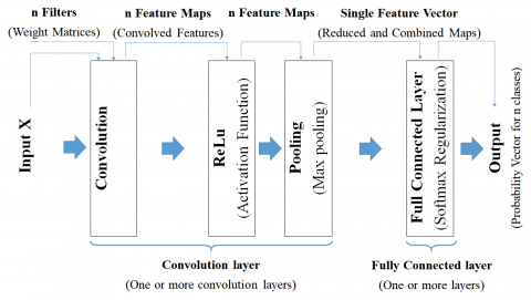
CNN network is a special FFNN with specific layers, used in general to deal with classification problem in imaging processing field. As illustrated in Figure 6, its basic architecture includes the convolution, the ReLU (Rectified Linear Unit) and the pooling layers in addition to the fully connected layer. The convolution layer receives input data (e.g. an image X) and filters (n different weight matrices), and transform data into feature maps (convolved features). In the ReLU layer, the activation function ReLU that is the most popular for deep neural networks [32], is then used. Besides, a max pooling function is commonly applied in the pooling layer to transform the feature maps into univariate vectors by reducing their sizes, and to combine these vectors to transform them into a single univariate one. Finally, the fully connected layer performs a softmax function regularization to generate a probability vector indicating the probability that X belongs to each of n classes. Note that a feature map is generated by convolving a filter over the input object (e.g. image X).
Figure 6. Basic CNN technique
Figure 7. Popular activation functions [32]
CNN network was designed to map image data to an output variable, and it works well for data with a spatial relationship. It uses a local connectivity between neurons (a neuron is only connected to nearby neurons in the next layer) allowing to significantly reduce the total number of parameters in the network [32]. However, CNN networks can be used to deal both with classification as well as regression problems.
Different activation functions are used in the literature. Among them Sigmoid, tanh, ReLU, Leaky ReLU, Maxout, ELU that are the most popular ones Figure 7.
The method Figure 8 we were adopted for forecasting COVID-19 Spread is composed out of different standard artifacts in ML/DL process. It is based on four main stages: data collection, data preprocessing, Models’ training and parametrization and models testing and validation.
Figure 8. Adopted method for forecasting COVID-19 spread
Figure 9. Occurrences preview of the used features in the COVID-19 prediction (Morocco)
Many datasets have been publically available on different sites such as WHO (World Health Organization), Kaggle, Github, Worldometers, and John Hopkins University to aid the fight against COVID-19 [33]. Our study relies on data from the European Center for Disease Prevention and Control (ECDC). The data is provided in a CSV format with 55 columns. Figure 9 presents a preview of four main columns corresponding to Morocco’s data from March to December. The values of new cases, total cases, new death and total death vary respectively from 0 to 6195, 0 to 417125, 0 to 92, and 0 to 6957.
This public dataset contains data around the world, and gives information about new confirmed cases, total confirmed cases, deaths, corresponding date, total tests, population density, as well as other potential variables.
For our study, we have selected only data related to Morocco’s case from February 07, 2020 to December 20 ,2020 for training and test set, we have also added data from December 21, 2020 to January 18, 2021 for the purpose of visual assessments of the performance of our models for the beginning of the year 2021. We also kept only features that are the most highly correlated variables to the targeted output (new confirmed cases) such as new confirmed cases and total deaths with respectively 100% and 96,17% as correlation values. For this purpose, we considered correlation percentages between the columns of the dataset, obtained using the Pearson correlation calculated as shown in Eq. (1). We, hence, kept four features (columns), notably those that showed a strong correlation between them, namely, new cases, total cases, new deaths, and total deaths. The date column was also kept as a line index.
$\boldsymbol{r}_{x y}=\frac{\sum_{i}^{n}\left(\boldsymbol{x}_{\boldsymbol{i}}-\overline{\boldsymbol{x}}\right)\left(\boldsymbol{y}_{\boldsymbol{i}}-\overline{\boldsymbol{y}}\right)}{\sqrt{\sum_{i}^{n}\left(\boldsymbol{x}_{\boldsymbol{i}}-\overline{\boldsymbol{x}}\right)^{2}} \sqrt{\sum_{i}^{n}\left(\boldsymbol{y}_{i}-\overline{\boldsymbol{y}}\right)^{2}}}$ (1)
where:
n : denotes the size of dataset,
x,y : are two columns of dataset,
xi,yi : are values of x and y indexed with i,
$\bar{x}, \bar{y}$ : are the mean of x and y respectively columns
Note that we have split this data into three datasets: confinement, deconfinement and hybrid datasets in order to then analyze the performance of the studied models while assessing the impact of the periods on their accuracy.
Data pre-processing is an important process needed to make collected data in an appropriate form in the way that it can readily and accurately be analyzed. It globally, consists of different tasks such data normalization, data filtering, data cleaning and data augmentation. In this context, after selecting data corresponding to Moroccan’s case and target periods, and also identifying the appropriate features as mentioned above, we have had to complete some data. For this purpose, we experimented two popular methods based respectively on Median value and Key Nearest Neighbor (KNN) algorithm before selecting the most appropriate one. We note that we have finally selected the first one (Median) in order to fill missing data.
For the sake of scale unification, the Min-Max scaler was also used in our experimentation to overcome noises during the learning process. Consequently, data like total cases and new cases that were respectively expressed in thousands and hundreds are transformed into data ranging from 0 to 1 using the min-max method, as shown in Eq. (2). It is worth noting that using this method is important since it allows the optimizer algorithms to generate the best weights that help to accelerate the learning process.
$x_{\text {scale }}=\frac{x_{i}-x_{\min }}{x_{\max }-x_{\min }}$ (2)
where:
xi : is the value of a feature x indexed with i before normalization,
xmin : is the minimum value of feature x,
xmax : is the maximum value of feature x,
xscale : is the new value of xi after normalization.
Besides, in the time-series problems, the model is trained and tested to learn from past features related to past time sequences (time lags) in such a way that it would be able to predict future ones related to a future time step. On the one hand, given the fact that analyzing COVID-19 data is a complex time-series problem due to the nature of the virus, which remains unrecognized and mutates rapidly, as well as the impact of the changing context, and on the other hand, for the sake of giving decision-makers enough time so that they can implement underlying strategies, we have organized our dataset by considering different time lags and 7 days as time step. Note that the time lag choice was constrained by the dataset size and that exploring different time lags will help seeking from which past time sequences, each of the elaborated models would be efficient and able to learn better, and then to give the most accurate predictions. Indeed, deep learning algorithms learn better when the data size is large. We have in our dataset (containing data of Morocco) nearly 345 days recorded. This size remains very insufficient and doesn’t allow to widely take advantage of the capabilities of deep learning algorithms. After trying several sizes of time lags in our practical study, we noticed a positive correlation between an increase in the number of time lag sequences and a gain in the model’s performance. Besides, we have seen that increasing the size of the time lags has had a negative impact because this number of sequences has decreased due to the small size of our dataset. This became harmful for our deep learning algorithms. It was therefore necessary to find the right size of the lags by taking into account the size of our dataset, and consequently find the related time step for which the model would be able to predict the targeted value. However, with an increasing amount of data, we think that it would be possible to increase the time lags size, and hence the time step for long-term predictions.
Finally, the data pre-processing stage gave rise to three datasets. These datasets: confinement, deconfinement, and hybrid, were obtained from our original dataset using the same scale of values (0 or 1) according to the Min-Max method, and converted into sequences using the m lags - n steps format. They respectively range from February 7 to June 15, June 16 to December 2, and February 7 to December 2, 2020. The ranges have been defined according to the best practices in data analysis. We have divided each dataset into 80% and 20%, respectively for the training set and the test set. Moreover, the DL models have been parametrized during the training stage while also considering large batch sizes in order to lead to the most accurate projections. After tuning different settings for our DL models, Adam optimizer has turned out to be the best optimizer and then, has been selected as a common parameter for all the proposed DL models. ADAM that works better than other stochastic optimizers in empirical experiments [34], would make the models able to learn fast. The tanh activation function has led to good fitting regarding the outcomes of the MSE regression loss function for all DL models, except the CNN model for which ReLU is best adapted.
Besides, all the designed models have to be fully trained and also tested using the test datasets in order to confirm their efficiency. For this purpose, we have used the most popular performance metrics used to evaluate ML and DL models results: MSE (Mean Square Error), RMSE (Root Mean Square Error), MAE (Mean Absolute Error), Max Error (ME) and R squared (R2). Their related formulas are given below.
$\mathrm{MSE}=\frac{1}{\mathrm{n}} \sum_{\mathrm{j}=1}^{\mathrm{n}}\left(\mathrm{y}_{\mathrm{j}}-\hat{\mathrm{y}}_{\mathrm{j}}\right)^{2}$ (3)
$\mathrm{MAE}=\frac{1}{\mathrm{n}} \sum_{\mathrm{j}=1}^{\mathrm{n}}\left|\mathrm{y}_{\mathrm{j}}-\hat{\mathrm{y}}_{\mathrm{j}}\right|$ (4)
$\mathrm{RMSE}=\sqrt{\frac{1}{\mathrm{n}} \sum_{\mathrm{j}=1}^{\mathrm{n}}\left(\mathrm{y}_{\mathrm{j}}-\hat{\mathrm{y}}_{\mathrm{j}}\right)^{2}}$ (5)
$\mathrm{ME}=\operatorname{Max}_{1 \leq j \leq n}\left|y_{j}-\hat{y}_{j}\right|$ (6)
$\mathrm{R} 2=1-\left(\frac{\mathrm{SSres}}{\mathrm{SStot}}\right)$ (7)
MSE is a default metric used to evaluate the most regression algorithms [35]. It measures the average squared errors (difference between the real y values and what is estimated $\hat{\mathrm{y}}$) [36]. A large MSE means a large error. However, this metric is sensitive to outliers and noisy data. RMSE is the square root of MSE [37] and is considered as the standard error deviation. It is useful to deal with high error issues and is a standard statistical metric used in meteorology, air quality, and climate research studies [38]. MAE measures the average of the absolute errors (absolute values corresponding to the differences between the real and the predicted values), whereas ME calculates the maximum residual error and highlights the worst error between the real and the predicted values. R2, also called the coefficient of determination, evaluates the rate between the residual sum of squares (SSres) and their total sum (SStot) and in other terms, the proportion of the outcome variance explained by the model. It indicates the efficiency of the model fitting, and ranges from 0 to 1. The closer to 1 it is, the better the model is [39].
Finally, note that all these different method stages were carried out and implemented using Python libraries, namely, Pandas, NumPy, SciPy and Matplotlib in a jupyter notebook, in addition to Scikit-learn (sklearn) and TensorFlow.
Our DL models have different architectures and different numbers of layers and neurons that were fixed after tuning different values. Details about the architectures and main parameters of each model that outperforms the other proposed ones for each explored dataset are given in Table 1. We respectively use CONV, GRU and FC terms to denote convolution, GRU and fully connected layers.
Table 1. Architecture and parameters of the best models
|
Datasets |
Confinement |
Deconfinement |
Hybrid |
|
Parameters |
RF |
CNN |
CNN |
|
Kernel-1D |
- |
2 |
2 |
|
Max Pooling-1D |
|
2 |
2 |
|
Layers |
- |
1 |
1 |
|
FC |
- |
127, 62, 7 |
111, 61, 7 |
|
Filters |
- |
255 |
249 |
|
Epocs |
- |
50 |
50 |
|
Activation Function |
- |
Relu |
Relu |
|
Regularization Function |
- |
dropout |
dropout |
|
Optimizer |
- |
Adam |
Adam |
|
Time Lag |
- |
7 |
7 |
|
Timestep |
- |
7 |
7 |
|
Batch Size |
- |
10 |
10 |
|
number of trees |
100 |
- |
- |
|
samples |
2 |
- |
- |
|
Leaf size |
1 |
- |
- |
Figure 10. CNN model architecture used
The structure of CNN models used in this paper is shown in Figure 10. We have tried several configurations. CNN-1D networks used in our document, having one convolution layer which contains filters ranging from 1 to 256, with a one-dimensional kernel of value equal to 2, and 3 FC layers. The neurons of the FC layers are varying between 1 and 127 for the first and the second layers. Whereas, the last one is the prediction layer that contains seven neurons. It is important to note here that the parameter setting of the layers related to our different studied models, has been made after successive experiments.
In this section, we present the results of four scenarios (corresponding to different time lags: 1, 2, 4 and 7 days) for each studied model, while giving information about the five-performance metrics MSE, RMSE, MAE, Max Error (ME) and R2. However, we interpret these results by referring to the RMSE metric that is a good measure of how accurately the model predicts the outcomes, since it gives higher weighting to the unfavorable conditions. Note that R2 is also a widely used metric. Nevertheless, it is not an appropriate indicator of how well the model fits the data [40]. A small value of R2 or a large one does not necessarily mean that the model is bad or that is automatically right [41]. Given this controversy around the goodness of R2 as an appropriate metric for identifying the best regression model [40, 42], we mainly use RMSE to compare our models in the rest of this document.
The best results metrics for each studied model and the corresponding time lag are shown in Table 2. We can notice that all the models well perform both at the test and training levels for the confinement, deconfinement and global context.
Table 2. Best metrics values per dataset and model
|
Dataset |
Model |
Data |
MSE |
RMSE |
MAE |
R2 |
Max Error |
|
Confinement |
CNN-1D (7-7) |
Training |
767.80 |
27.71 |
19.67 |
0.81 |
112.53 |
|
Test |
1071.74 |
32.74 |
22.91 |
0.65 |
116.28 |
||
|
MLP (7-7) |
Training |
1170.66 |
34.21 |
25.85 |
0.70 |
130.28 |
|
|
Test |
1639.4 |
40.49 |
30.25 |
0.46 |
175.27 |
||
|
LSTM (7-7) |
Training |
1374.58 |
37.08 |
26.90 |
0.65 |
162.89 |
|
|
Test |
1419.16 |
37.67 |
26.64 |
0.53 |
165.5 |
||
|
GRU (7-7) |
Training |
1304.83 |
36.12 |
26.32 |
0.67 |
150.00 |
|
|
Test |
1399.21 |
37.41 |
26.97 |
0.54 |
152.1 |
||
|
RF (1-7) |
Training |
198.8 |
14.09 |
9.99 |
0.95 |
48.13 |
|
|
Test |
1005.07 |
31.7 |
20.62 |
0.69 |
108.56 |
||
|
LR (1-7) |
Training |
1611.67 |
40.14 |
28.92 |
0.57 |
172.97 |
|
|
Test |
1636.02 |
40.45 |
29.22 |
0.49 |
161.32 |
||
|
Deconfinement |
CNN-1D (7-7) |
Training |
178368.53 |
422.34 |
302.63 |
0.93 |
1971.83 |
|
Test |
143655.3 |
379.02 |
282.26 |
0.94 |
1264.22 |
||
|
MLP (7-7) |
Training |
196442.41 |
443.22 |
321.21 |
0.92 |
1988.56 |
|
|
Test |
158162.61 |
397.7 |
301.71 |
0.94 |
1235.08 |
||
|
LSTM (7-7) |
Training |
427212.28 |
653.61 |
478.16 |
0.82 |
2350.97 |
|
|
Test |
367080.25 |
605.87 |
463.44 |
0.86 |
1819.87 |
||
|
GRU (7-7) |
Training |
289559.72 |
538.11 |
385.98 |
0.88 |
2260.06 |
|
|
Test |
229082.69 |
478.63 |
369.59 |
0.91 |
1639.66 |
||
|
RF (4-7) |
Training |
45347.12 |
212.94 |
141.6 |
0.98 |
1032.71 |
|
|
Test |
226823.06 |
476.26 |
314.79 |
0.9 |
1778.46 |
||
|
LR (7-7) |
Training |
185594.42 |
430.8 |
310.15 |
0.92 |
2070.72 |
|
|
Test |
165405.69 |
406.7 |
309.26 |
0.94 |
1361.83 |
||
|
Hybrid |
CNN-1D (7-7) |
Training |
111935.71 |
334.57 |
198.78 |
0.96 |
2075.90 |
|
Test |
102634.32 |
320.37 |
196.64 |
0.96 |
1368.6 |
||
|
MLP (7-7) |
Training |
139185.39 |
373.08 |
236.09 |
0.95 |
2394.55 |
|
|
Test |
116182.73 |
340.86 |
226.21 |
0.95 |
1458.49 |
||
|
LSTM (7-7) |
Training |
244480.97 |
494.45 |
303.62 |
0.91 |
2273.87 |
|
|
Test |
195677.08 |
442.35 |
288.6 |
0.92 |
1816.34 |
||
|
GRU (7-7) |
Training |
275617.34 |
524.99 |
312.80 |
0.89 |
2541.39 |
|
|
Test |
213759.45 |
462.34 |
296.95 |
0.91 |
1896.49 |
||
|
RF (7-7) |
Training |
24061.55 |
155.11 |
84.71 |
0.99 |
869.32 |
|
|
Test |
137890.36 |
371.34 |
202.44 |
0.94 |
1860.75 |
||
|
LR (4-7) |
Training |
162381.88 |
402.96 |
244.86 |
0.94 |
2177.81 |
|
|
Test |
148269.31 |
385.06 |
248.01 |
0.93 |
2575.24 |
Figure 11. RF 1-7 Curves of prediction results in confinement period
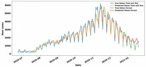
Figure 12. CNN 7-7 Curves of prediction results in confinement period
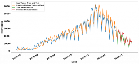
Figure 13. CNN 7-7 curves of prediction results in deconfinement period
Figure 14. MLP 7-7 curves of prediction results in deconfinement period
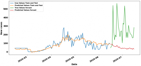
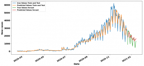
Figure 15. CNN 7-7 curves of prediction results in hybrid period
Figure 16. MLP 7-7 curves of prediction results in hybrid period
In the containment period, the LR has the best result RMSE value equal to 31.7 with 1 lag and 7 steps which is very close to the CNN’RMSE value equal to 32.74 with 7 lags. Figure 11 and Figure 12 show their training/testing curves. In the context of deconfinement, we observe that the CNN model surpasses the rest of the models with an RMSE value of 379.02 and 7 as a time lag, the MLP Model with 7 lags also has a good value about 397.7. Figure 13 and Figure 14 respectively show their training /testing curves. For the hybrid (confinement and deconfinement put together) case, CNN with 7 lags models outperform the other ones with RMSE value of 320.37, although the MLP with 7 lags is also doing well with RMSE about 340.86. The training and testing curves are shown in Figure 15 and Figure 16.
Table 3. Best metrics related to three periods
|
Period |
Model |
Data |
RMSE |
R2 |
NRMSE |
|
Confinement |
RF (1-7) |
Train |
14.09 |
0.95 |
0.05 |
|
Test |
31.7 |
0.69 |
0.11 |
||
|
Deconfinement |
CNN-1D (7-7) |
Train |
422.34 |
0.93 |
0.07 |
|
Test |
379.02 |
0.94 |
0.06 |
||
|
Global |
CNN-1D (7-7) |
Train |
334.57 |
0.96 |
0.05 |
|
Test |
320.37 |
0.96 |
0.05 |
In short, Table 3 highlights the three models with the best and most interesting performances, in particular those with the top (lowest) RMSE measure, for each of the periods studied.
Besides, even if the RMSE metric is a good measure of how accurately the model predicts the response, it is still difficult to be interpreted. In this section, we use normalize the RMSE, the normalized RMSE (NRMSE) is the rate of the RMSE value and the range (the maximum value minus the minimum value) of observation values. The RMSE does not allow to compare models coming from different datasets, it suits to say which is the best model among models having been trained on the same Dataset. In order to compare the best models coming from the three periods (confinement, deconfinement and hybrid), we are going to use the NRMSE, as shown in Table 3, indeed the lower the NRMSE the better the model, if we have to classify the models according to their performances on the test set, we have as first model the CNN (7-7) of the global dataset with a NRMSE equal to 0.05, as second-best model we have the CNN (7-7) of the deconfinement with a NRMSE equal to 0.06 and finally the RF (1-7) model of the deconfinement with a NRMSE equal to 0.11. We can also appreciate the performance of the models by examining the best prediction curves, indeed, if we compare the containment, unconfinement and hybrid curves respectively in Figure 11, Figure 13 and Figure 15, we also notice that on the figure CNN(7-7) of the hybrid period, the prediction curve in orange color is very close to the actual values in blue color compared to the CNN(7-7) curve of the deconfinement period, this comparison remains valid for the deconfinement curves of the CNN (7-7) compared to the containment curves of the RF model (1-7). We can therefore say that, CNN was the best performing on this paper, whether for the containment period (where its RMSE value is quite close to the best one-unit ready model), the deconfinement period or the hybrid period. Although neglected by researchers for regression tasks because of its affinity with image processing, we find that the CNN for the prediction of new cases of COVID-19 is the most relevant for models such as the LSTM which is often better suited for sequential data processing. period), and the incoherent sizes of data since we have more confinement data than deconfinement one. We can therefore say that the CNN has been the best performer on this paper, whether for the containment period (where its RMSE value is quite close to the best model at a ready value), deconfinement or the hybrid period. Although neglected by researchers for regression tasks because of its affinity with image processing, we find that the CNN for the prediction of new cases of COVID-19 is the most relevant for models such as LSTM which is often better suited for sequential data processing.
The aim of this paper was on one hand, to evaluate the efficiency of the ML and the DL models as well as the impact of the time lag size and the confinement/deconfinement context for predicting the propagation of COVID-19 in the world by experimenting Morocco’s case, and on the other hand, to estimate the ability of these AI techniques to provide mean-term forecasts from small datasets. The long-term and the mean-term predictions are necessary to give decision-makers enough time to take appropriate decisions, such as short-time confinement, provisioning required resources (beds in hospitals, test kits…), and selecting appropriate health protocols, in order to stop the spread of COVID-19 in the world.
According to the results of this work, we outline the efficiency of the DL models compared to the ML ones. We can indeed conclude that these last ones aren’t suitable for COVID-19 spread prediction, which is a complex time-series problem. However, the first ones provide promising results. The CNN model has especially outperformed or provided results that were very close to those provided by all the other models for the three studied periods. Although the CNN model is deemed more suitable for image processing and classification issues, the results of this work have highlighted its efficiency for complex regression problems like COVID-19 outbreak forecasting with different datasets sizes. Note that the RF and MLP models are also suitable and it would be interesting to investigate these two models further.
After experimenting our models to perform predictions for the next 7 days, the ones with long time lags (7 days in both deconfinement and hybrid cases) have provided good and promising results in term of NRMSE. Therefore, we conclude that COVID-19 spread prediction is indeed a mean-term time-series problem that requires learning from data related to several previous days. This can be explained by the virus incubation period that ranges from 1 to 14 days with an average of 5 to 6 days. In addition to this, we think that DL models could provide good long-term predictions (for over a week) if larger datasets are used, since DL models are generally designed to learn from huge datasets.
When we examine our results to assess the impact of the confinement and the deconfinement on the projections accuracy, we can see that the COVID-19 outbreak prediction is a context-aware problem, thus other context parameters such as the test kits, the asymptomatic cases and the region density, are required for better learning and projections that are more accurate.
Finally, we think that the findings of this work could be useful in other epidemic contexts and for designing DL models that help to anticipate the spread of viruses in other countries. However, our models could be optimized by experimenting larger and richer datasets. This help to have a perfect balance between confinement and deconfinement data, and to take account of other features defining crucial context parameters, while evaluating the impact of the context on the predictions’ accuracy and the projections of different countries.
This paper was written within the scope of a COVID-19 project supported by the supervisory ministry MENFPESRS and the CNRST of Morocco with the aim of prevention and forecast the spread of the COVID-19 pandemic.
[1] Wiens, J., Shenoy, E.S. (2018). Machine learning for healthcare: on the verge of a major shift in healthcare epidemiology. Clinical Infectious Diseases, 66(1): 149-153. https://doi.org/10.1093/cid/cix731
[2] World Health Organization. (2020). Coronavirus disease 2019 (COVID-19): situation report, 82. https://www.who.int/docs/default-source/coronaviruse/situation-reports/20200816-covid-19-sitrep-209.pdf?sfvrsn=5dde1ca2_2.
[3] Pinter, G., Felde, I., Mosavi, A., Ghamisi, P., Gloaguen, R. (2020). COVID-19 pandemic prediction for Hungary; a hybrid machine learning approach. Mathematics, 8(6): 890. https://doi.org/10.3390/math8060890
[4] Koolhof, I.S., Gibney, K.B., Bettiol, S., Charleston, M., Wiethoelter, A., Arnold, A.L., Firestone, S.M. (2020). The forecasting of dynamical Ross River virus outbreaks: Victoria, Australia. Epidemics, 30: 100377. https://doi.org/10.1016/j.epidem.2019.100377
[5] Liang, R., Lu, Y., Qu, X., Su, Q., Li, C., Xia, S., Niu, B. (2020). Prediction for global African swine fever outbreaks based on a combination of random forest algorithms and meteorological data. Transboundary and emerging diseases, 67(2): 935-946. https://doi.org/10.1111/tbed.13424
[6] Tapak, L., Hamidi, O., Fathian, M., Karami, M. (2019). Comparative evaluation of time series models for predicting influenza outbreaks: Application of influenza-like illness data from sentinel sites of healthcare centers in Iran. BMC Research Notes, 12(1): 1-6. https://doi.org/10.1186/s13104-019-4393-y
[7] Anno, S., Hara, T., Kai, H., Lee, M.A., Chang, Y., Oyoshi, K., Tadono, T. (2019). Spatiotemporal dengue fever hotspots associated with climatic factors in taiwan including outbreak predictions based on machine-learning. Geospatial Health, 14(2): https://doi.org/10.4081/gh.2019.771
[8] Chenar, S.S., Deng, Z. (2018). Development of artificial intelligence approach to forecasting oyster norovirus outbreaks along Gulf of Mexico coast. Environment International, 111: 212-223. https://doi.org/10.1016/j.envint.2017.11.032
[9] Chenar, S.S., Deng, Z. (2018). Development of genetic programming-based model for predicting oyster norovirus outbreak risks. Water Research, 128: 20-37. https://doi.org/10.1016/j.watres.2017.10.032
[10] Muurlink, O.T., Stephenson, P., Islam, M.Z., Taylor-Robinson, A.W. (2018). Long-term predictors of dengue outbreaks in Bangladesh: A data mining approach. Infectious Disease Modelling, 3: 322-330. https://doi.org/10.1016/j.idm.2018.11.004
[11] Ardabili, S.F., Mosavi, A., Ghamisi, P., Ferdinand, F., Varkonyi-Koczy, A.R., Reuter, U., Atkinson, P.M. (2020). Covid-19 outbreak prediction with machine learning. Algorithms, 13(10): 249. https://doi.org/10.3390/a13100249
[12] Ndiaye, B.M., Tendeng, L., Seck, D. (2020). Analysis of the COVID-19 pandemic by SIR model and machine learning technics for forecasting. arXiv preprint arXiv:2004.01574.
[13] Yadav, R.S. (2020). Data analysis of COVID-2019 epidemic using machine learning methods: a case study of India. International Journal of Information Technology, 12: 1321-1330. https://doi.org/10.1007/s41870-020-00484-y
[14] Zou, D., Wang, L., Xu, P., Chen, J., Zhang, W., Gu, Q. (2020). Epidemic model guided machine learning for COVID-19 forecasts in the United States. medRxiv.
[15] Singh, K.K., Kumar, S., Dixit, P., Bajpai, M.K. (2020). Kalman filter based short term prediction model for COVID-19 spread. Applied Intelligence, 1-13. https://doi.org/10.1007/s10489-020-01948-1
[16] Yeşilkanat, C.M. (2020). Spatio-temporal estimation of the daily cases of COVID-19 in worldwide using random forest machine learning algorithm. Chaos, Solitons & Fractals, 140: 110210. https://doi.org/10.1016/j.chaos.2020.110210
[17] Bouhamed, H. (2020). Covid-19 cases and recovery previsions with deep learning nested sequence prediction models with long short-term memory (LSTM) architecture. Int. J. Sci. Res. in Computer Science and Engineering, 8(2): 10-15.
[18] Chimmula, V.K.R., Zhang, L. (2020). Time series forecasting of COVID-19 transmission in Canada using LSTM networks. Chaos, Solitons & Fractals, 135: 109864. https://doi.org/10.1016/j.chaos.2020.109864
[19] Liu, B., Yan, S., Li, J., Qu, G., Li, Y., Lang, J., Gu, R. (2019). A sequence-to-sequence air quality predictor based on the n-step recurrent prediction. IEEE Access, 7: 43331-43345. https://doi.org/10.1109/ACCESS.2019.2908081
[20] Hao, S., Lee, D. H., Zhao, D. (2019). Sequence to sequence learning with attention mechanism for short-term passenger flow prediction in large-scale metro system. Transportation Research Part C: Emerging Technologies, 107: 287-300. https://doi.org/10.1016/j.trc.2019.08.005
[21] Murdoch, W.J., Singh, C., Kumbier, K., Abbasi-Asl, R., Yu, B. (2019). Definitions, methods, and applications in interpretable machine learning. Proceedings of the National Academy of Sciences, 116(44): 22071-22080. https://doi.org/10.1073/pnas.1900654116
[22] Sharma, S. (2017). Artificial Neural Network (ANN) in Machine Learning. Available: https://www.datasciencecentral.com/profiles/blogs/artificial-neural-network-ann-in-machine-learning.
[23] Zou, K.H., Tuncali, K., Silverman, S.G. (2003). Correlation and simple linear regression. Radiology, 227(3): 617-628. https://doi.org/10.1148/radiol.2273011499
[24] Mendes-Moreira, J., Jorge, A.M., de Sousa, J.F., Soares, C. (2012). Comparing state-of-the-art regression methods for long term travel time prediction. Intelligent Data Analysis, 16(3): 427-449. https://doi.org/10.3233/IDA-2012-0532
[25] Mosavi, A., Ozturk, P., Chau, K.W. (2018). Flood prediction using machine learning models: Literature review. Water, 10(11): 1536. https://doi.org/10.3390/w10111536
[26] Chakure, A. (2020). Random Forest Regression. Available: https://towardsdatascience.com/random-forest-and-its-implementation-71824ced454f.
[27] Terry-Jack, M. (2019). Deep Learning: Feed Forward Neural Networks (FFNNs), Available: https://medium.com/@b.terryjack/introduction-to-deep-learning-feed-forward-neural-networks-ffnns-a-k-a-c688d83a309d.
[28] Nguyen, G., Dlugolinsky, S., Bobák, M., Tran, V., García, Á.L., Heredia, I., Hluchý, L. (2019). Machine learning and deep learning frameworks and libraries for large-scale data mining: a survey. Artificial Intelligence Review, 52(1): 77-124. https://doi.org/10.1007/s10462-018-09679-z
[29] Hochreiter, S., Schmidhuber, J. (1997). Long short-term memory. Neural computation, 9(8): 1735-1780. https://doi.org/10.1162/neco.1997.9.8.1735
[30] Ronaghan, S. (2018). Deep Learning: Common Architectures. Available: https://mc.ai/deep-learning-common-architectures/.
[31] Dey, R., Salem, F.M. (2017). Gate-variants of gated recurrent unit (GRU) neural networks. In 2017 IEEE 60th International Midwest Symposium on Circuits and Systems (MWSCAS), 1597-1600. https://doi.org/10.1109/MWSCAS.2017.8053243
[32] Emmert-Streib, F., Yang, Z., Feng, H., Tripathi, S., Dehmer, M. (2020). An introductory review of deep learning for prediction models with big data. Frontiers in Artificial Intelligence, 3: 4. https://doi.org/10.3389/frai.2020.00004
[33] Shuja, J., Alanazi, E., Alasmary, W., Alashaikh, A. (2020). Covid-19 open source data sets: A comprehensive survey. Applied Intelligence, 51: 1296-1325. https://doi.org/10.1007/s10489-020-01862-6
[34] Kingma, D.P., Ba, J. (2014). Adam: A method for stochastic optimization. arXiv preprint arXiv:1412.6980.
[35] Kathuria, C. (2019). Regression—Why Mean Square Error? Available: https://towardsdatascience.com/https-medium-com-chayankathuria-regression-why-mean-square-error-a8cad2a1c96f.
[36] Binieli, M. (2018). Machine learning: an introduction to mean squared error and regression lines. # MATHEMATICS, Free Code Camp.
[37] Bratsas, C., Koupidis, K., Salanova, J.M., Giannakopoulos, K., Kaloudis, A., Aifadopoulou, G. (2020). A comparison of machine learning methods for the prediction of traffic speed in urban places. Sustainability, 12(1): 142. https://doi.org/10.3390/su12010142
[38] Chai, T., Draxler, R.R. (2014). Root mean square error (RMSE) or mean absolute error (MAE)? Arguments against avoiding RMSE in the literature. Geoscientific Model Development, 7(3): 1247-1250. https://doi.org/10.5194/gmd-7-1247-2014
[39] Vedova, C.D. (2018). Régression linéaire simple : le R2, info ou intox ? Available: https://statistique-et-logiciel-r.com/regression-lineaire-simple-le-r%C2%B2-info-ou-intox/.
[40] Moksony, F., Heged, R. (1990). Small is beautiful. The use and interpretation of R2 in social research. Szociológiai Szemle, Special issue, 130-138. https://doi.org/10.11606/issn.2237-4485.lev.2011.132282
[41] Figueiredo Filho, D.B., Júnior, J.A.S., Rocha, E.C. (2011). What is R2 all about? Leviathan (São Paulo), (3): 60-68.
[42] Anderson-Sprecher, R. (1994). Model comparisons and R2. The American Statistician, 48(2): 113-117. https://doi.org/10.1080/00031305.1994.10476036