Nadia Zerguine* | Mohammed Mostefai | Zibouda Aliouat | Yacine Slimani
© 2020 IIETA. This article is published by IIETA and is licensed under the CC BY 4.0 license (http://creativecommons.org/licenses/by/4.0/).
OPEN ACCESS
Mobile ad hoc networks (MANETs) consist of self-configured mobile wireless nodes capable of communicating with each other without any fixed infrastructure or centralized administration using the medium radio. Wireless technology is based on standard IEEE.802.11. The IEEE 802.11 Distributed Coordination Function (DCF) MAC layer uses the Binary Exponential Backoff (BEB) algorithm to deal with wireless network collisions. BEB is considered effective in reducing the probability of collisions but at the expense of numerous network performance measures, such as throughput and packets delivery ratio, mainly in high traffic load. Deep Reinforcement Learning (DRL) is a DL technique in which an agent can achieve a goal by interacting with the environment. In this paper, using one of the DRL models, we propose Q-learning (QL) to optimize MAC protocols' performance based on the contention window (CW) in MANETs. The intelligent proposed MISQ takes into account the number of packets to be transmitted and the collisions committed by each station to select the appropriate contention window. The performance of the proposed mechanism is evaluated by using in-depth simulations. The outputs indicate that the intelligent proposal mechanism learns various MANETS environments and optimizes performance over standard MAC protocol. The performance of MISQ is evaluated in various networks with throughput, channel access delay, and packets delivery rate as performance measures.
DCF, deep reinforcement learning, CW, IEEE 802.11, MAC protocol, MANET, Q-learning
The field of communications has experienced remarkable success and growth in recent years due to technological advances, and particularly the emergence of wireless technology. The latter enables the implementation of wireless communications in mobile environments, which provide a great degree of convenience of use. In fact, mobile ad hoc networks (MANETs) are a modern model for mobile networks, they are local networks where inter-station communication is carried out by radio frequencies, designed by the interconnection of various kinds of devices nodes, and does not require any fixed infrastructure or centralized control. The topology of this kind of networks is often unstable and changeable due to the mobility of nodes. In addition, the radio channel and the bandwidth available for communication in such networks are limited. Admission to the common channel should be handled in such a way that all stations receive their share of the amount of available bandwidth. The bandwidth sharing must be fair between all stations, efficient, and without consequences on network resources. This admission, is carried out by the protocol MAC (Medium Access Control) and, because of all the challenges of MANETs, a huge dilemma is the development of an easy, efficient and equitable shared medium access control system.
The IEEE 802.11 MAC protocol is the standard deployed for untethering (wireless) LAN communication, although, it belongs to the same standard family as Ethernet, it has a very different architecture and medium access protocol. The IEEE 802.11 MAC Protocol supports some wireless multi-hop ad hoc networks, even it was not built for wireless mobile ad hoc networks where multi-hop connectivity is a primary feature [1]. Two key metrics are used to measure the efficiency of the MAC protocol: the probability of collision and fairness in allocating the channel to contending stations. IEEE 802.11 is trying to solve the collision problem by following the Binary Exponential Backoff (BEB) algorithm. The BEB scheme is the typical kernel Carrier Sense Multiple Access/Collision Avoidance (CSMA/CA) framework implemented in IEEE 802.11 DCF [2]. This backoff framework, used in the most contention-based wireless medium access protocols, is generally adapted from ethernet networks where there is no non-uniform media activity. The BEB method of providing equal medium access in wired networks thus becomes the source of inequality in wireless networks; it suffers from both fairness and efficiency. The inequality of the MAC layer affects the actions of higher layer protocols.
Over and above that, nowadays, deep learning (DL) has attracted much attention from the research community and industry because to the successful applications in different research fields, such as speech recognition, natural language processing, and computer vision. This attention has led to the development of using deep learning (DL) in wireless communications technologies to benefit from artificial intelligence's advantages in this field. DL principles have a longstanding background in wireless networks and have achieved much success, especially in upper communication layers, such as in cognitive radio networks (CRNs) and resource management of the MAC layer [3]. Many researchers believe that the introduction of DL into wireless networks can optimize the performance of these networks. A DL technique is deep reinforcement learning (DRL) which is motivated by behavioral sensitivity and the ideology of control. An agent DRL achieves a goal by communicating with its environment [4, 5]. DRL uses specific learning models, including Markov Decision Process (MDP), Partially Observed MDP (POMDP), and Q-learning (QL) [6]. QL is inspired by behavior, allowing discovering an optimal strategy of action for any finite MDP, mainly when the environment is unknown [7].
In this paper, we apply Q-learning-based reinforcement learning to learn the optimal backoff scheme in contention-based MAC protocol (without any access point) to improve network channel usage and the CSMA/CA performance in the MANETs. Unlike the classic Binary Exponential Backoff (BEB) (introduced in the next section), which only takes into account the information of success or collision transmission to initialize or increase the CW respectively, the proposal also takes into account the number of packets to be transmitted (for example, high or low) and the number of collisions made by the station, to select the appropriate CW. The results of the various simulations show that the proposed algorithm “intelligent mechanism of CW selection based on Q-learning (MISQ)” achieves a better throughput, an acceptable MAC layer access delay, and a delivered packet rate more significant than that of the BEB used in the IEEE802.11 DCF standard.
The rest of the paper is organized as follows: Section 2 presents the related work. Section 3 discusses the Markov decision process and reinforcement learning. The main part of this paper, the introduction of Q-learning, is provided in section 4 to optimize the contention window. The different simulations and results obtained are presented in section 5. Finally, section 6 concludes this work.
Binary Exponential Backoff (BEB), The Distributed Coordination Function (DCF) is the basic MAC of the IEEE 802.11 WLAN protocol. DCF is essentially a CSMA/CA (Carrier Sense Multiple Access with Collision Avoidance) mechanism with a BEB (Binary Exponential Backoff) algorithm [8]. This algorithm is used to push the station to delay access to the shared transmission channel for a random period of time [9]. The BEB algorithm operates according to the two resulting states after data transmission. If the data transmitted by a source station is received correctly by a destination station, then a transmission success is concluded, otherwise, a transmission failure is then detected. BEB resets the contention window CW to its initial value CWminin case of success, and doubles the CW in case of failure until maximum number CWmax is reached. once the number of retransmissions Rmax allowed for a data packet is reached, the data packet will be discarded, and an attempt to transmit the next packet is initiated from CWmin. Therefore, A station that succeeds in transmitting will likely have the channel in the next contention. A binary exponential interrupt period called backoff counter is randomly selected in [0, CW-1]; it is decreased when the channel is detected inactive. The station begins transmitting when the backoff timer expires. BEB is less effective when the number of stations becomes more significant [10, 11]. A short backoff time induces a heavy load on the channel with a low probability of successful transmission. However, a very long backoff time triggers channel inactivity. An adequate backoff mechanism is one that provide high throughput, more fairness, less delay, and more reliability. BEB calculates the contention window according to the two cases:
$C W_{n e w}=\left\{\begin{array}{ll}\left.\operatorname{Min}\left(\left(C W_{\text {cur }} * 2\right)+1, C W_{\max }\right)\right) & \text { collide } \\ C W_{\min } & \text { succeed }\end{array}\right.$ (1)
Cognitive Backoff Mechanism (CB), proposed by Shahin et al. [12], a mechanism that adaptively determines the CW to effectively avoid collision with high throughput and low transmission delay. In CB mechanism, the technique used in case of a successful transmission is identical to that used in BEB. Differently in case of a collision, CB mechanism updates the CW based on a measured conditional collision probability pck, backoff stages i, and an optimally defined backoff factor, (CWmin+1)(pck + 1). CB mechanism calculates the CW as follows:
$C W_{n e w}=\left\{\begin{array}{lr}\min \left(\left(2^{i}\left(C W_{\min }+1\right)^{(\mathrm{pck}+1)}-1\right), C W_{\max }\right)& \text { collide } \\ C W_{\min } & \text { succeed }\end{array}\right.$ (2)
Based on simulations, CB offers better performance than BEB in terms of throughput, delay, and fairness.
Centralized Contention Window Optimization with DRL (CCOD), proposed by Wydmański et al. [13], a method of applying DRL in multichannel networks that supports two trainable algorithms, having the task of optimizing the saturation rate of 802.11ax networks by correctly predicting CW values while keeping computational cost low.
Intelligent QL-Based Resource Allocation (iQRA), proposed by Ali et al. [14], an intelligent resource allocation mechanism based on QL was proposed for access to MAC layer channels in dense WLANs. The simulations have shown that compared to conventional non-intelligent MAC protocols, the performance of the iQRA results in better throughput, channel access delay, and fairness.
An MDP is a mathematic tool that allows modeling RL agents. It is defined as a quadruple MDP = (S, A, R, T) [15], where S represents all states of the system in which the process operates and A is the set of all possible actions that control the dynamics of the state. R is the reward function S×A→R, obtained by performing action a in state s and T is the transition probability function S×T×S→[0, 1], where T[s' |s, a] is the transition probability from the current state $s \in S$ to $s^{\prime} \in S$ after the action $a \in A$ is taking. The decision policy π maps the set of states S on the set of actions A: $\pi: S \rightarrow A$. Specifically, suppose that the environment is a stochastic system with discrete-time and finite states. Let S = (s1, s2, …; sn) be the state space S and A = (a1, a2, …, am) the action space A. If at episode i, the RL agent is on a state $s_{i} \in S$, it chooses the action $a_{i} \in A$, according to the policy π in order to interact with its environment. Then it passes to the state $s_{i} \in S$ with a probability $P\left(s^{\prime} \mid s, a\right)$ providing to the agent a return reward noted $r_{i}(s, a)$. The process is then recycled. The objective of the RL agent is to maximize the reward or the expected updated state value in the more or less long term, taking less and less account of the future using a coefficient γ$\in$ [0, 1], which is represented by:
$V^{\pi}(s)=R(s, a)+\gamma \sum_{s^{\prime} \in S} P\left(s^{\prime} \mid s, a\right) V^{\pi}\left(s^{\prime}\right)$ (3)
where, $R(s, a)=E\{r(s, a)\}$ is the average value of the reward r(s, a) and γ is the discount factor that allows modulating the importance of the expected future rewards. A factor equals to 0 will cause the agent to consider the last rewards, while a factor closes to 1 will cause the agent to consider long-term rewards as much as short-term.
A policy $V^{*}(s)$ is considered to be the optimal policy if and only if: $V^{*}(s) \geq V^{\pi}(s)$ for each $s \in S\left(V^{*}(s)=\max V^{\pi}(s)\right.$. The Eq. (3) can be rewritten recursively as the Bellman equation:
$V^{*}(s)=R(s, a)+\gamma \max _{a \in A(s)} \sum_{s^{\prime} \in S} P\left(s^{\prime} \mid s, a\right) V^{*}\left(s^{\prime}\right)$ (4)
Q-learning [16] is part of the model-free RL methods. It is about learning through experience what actions to take based on the current state. Q-learning attempts to determine the policy π, in the absence of the probability transition function and the reward function. In Q-learning, the policies and the value function are represented by a matrix indexed by state-action pairs. Formally, for each state s and action a, another quantity Q (s, a) obtained from V(s) [17], can be used. It will provide the "quality" of the action taken in the state.
The value Q under the policy π is defined as being:
$Q^{\pi}(s, a)=R(s, a)+\gamma \sum_{s^{\prime} \in S} P\left(s^{\prime} \mid s, a\right) V^{\pi}\left(s^{\prime}\right)$ (5)
Let $Q^{*}(s, a)=Q^{\pi^{*}}(s, a)=\max _{\pi} Q^{\pi}(s, a)$ being the optimal action function under the π policy, the optimal value function is rewritten using Q* (Bellman's equation) as:
$V^{*}(s)=\max _{a \in A(s)}\left(Q^{*}(s, a)\right)$ (6)
The optimal policy π is expressed:
$\pi^{*}=\mathrm{a}^{*}=\underset{a \in A(s)}{\operatorname{argmax}}\left(Q^{*}(s, a)\right)$ (7)
The value function of the optimal action Q∗ is the unique solution of Bellman's equation:
$Q^{*}(s, a)=R(s, a)+\gamma \sum_{s^{\prime} \in S} P\left(s^{\prime} \mid s, a\right) \max _{a^{\prime} \in A\left(s^{\prime}\right)} Q^{*}\left(s^{\prime}, a^{\prime}\right)$ (8)
The Q-learning algorithm looks for an approximation of Q* as a fixed point of the previous equation, by writing:
$Q_{t+1}\left(s_{t}, a_{t}\right)=Q_{t}\left(s_{t}, a_{t}\right)+\alpha \Delta Q_{t}\left(s_{t}, a_{t}\right)$ (9)
where, α$\in$ [0.1] is the learning rate, which determines the extent to which the new information acquired will replace the old information. A learning rate of 0 will not learn the agent anything, while a learning rate of 1 will only make it consider the most recent information.
Learning occurs rapidly based on an improved learning estimate ∆ called the temporal difference, expressed as:
$\Delta Q_{t}\left(s_{t}, a_{t}\right)=\left[r\left(s_{t}, a_{t}\right)+\gamma \max _{a^{\prime} \in A(s)} Q_{t}\left(s_{t+1}, a_{t}^{\prime}\right)-Q_{t}\left(s_{t}, a_{t}\right)\right]$ (10)
In the next section, we discuss the CW optimization algorithm concerning channel access delay, delivered packet rate, and throughput as an MDP. Our goal is to achieve an optimal channel access policy while correctly defining the reward function and the RL algorithm.
Packet collisions occur when multiple stations access the channel simultaneously. So, one of the goals of the contention-based MAC protocol is to avoid collisions. The station must therefore check the state of the channel to avoid collisions. A backoff mechanism is required for transmission after a certain delay when the channel is occupied. Determining the duration of the backoff requires a CW, and the efficiency of access to the channel is determined by the correct selection of the size of the CW. Although it is challenging to design an optimal channel access mechanism, it’s essential to choose an appropriate CW method. Thus, we adopted a CW selection scheme based on Q-learning, while defining a reward function to be maximized when the number of collisions or the number of packets generated by the station is important for quick channel access. The state-space contains the CW sizes according to the random exponential backoff binary scheme for each situation S, where S denotes success transmission or collision. Actions determine CW size in stage k from stage k-1. In this section, we discuss the defined reward function and the algorithm used to enable the agent to learn the optimal contention window selection policy. Channel access delay and throughput are two critical issues for wireless networks. Therefore, it would not be desirable to minimize the access time at the cost of an unacceptable throughput.
4.1 Reward function
The reward expresses the goal of a QL algorithm. In our proposition, depending on the both situations, the Q-learning agent selects a CW that maximizes the reward in state si. The reward function comprises two components, the first one considers the collisions Ck carried out by the station si in an episode k (We designate by episode the time since the packet is queued until its successful transmission or rejection after the number of allowed retransmissions is reached). The second component analyses the information Tk of the packet's number to be transmitted generated by the station si. The transmission queue occupancy rate of station siis defined as:
$T_{k}=\left(\frac{N B P_{k}}{Q u e u e S i z e}\right) * 100$ (11)
where, NBPk represents the number of packets in the si station's queue, in episode k, QueueSize is the queue size.
The rate of collisions committed by the station si in an episode k is as follows:
$C_{k}=\frac{\sum_{i=0}^{k} \operatorname{col}_{i}}{\operatorname{Rmax}} * 100$ (12)
where, coli is a collision of packet transmission by the station si, and Rmax is the number of retransmissions allowed for a packet.
A distinction between the two components of the reward is made by a fitness function which calculates the collision/ queue occupancy ratio as follows:
Fitness $=\alpha T_{k}+(1-\alpha) C_{k}$ (13)
Thus, the computation of the reward function is performed as:
$R_{T}=\left\{\begin{array}{cc}\frac{C_{k}}{\operatorname{Rmax}} \text { if fitness }>\text { threshold and high } T_{k} & \text { collide } \\ \frac{N B P_{k}}{\text { Queuesize }} \text { if fitness }<\text { threshold and high } T_{k} & \text { succeed } \\ 0 & \text { else }\end{array}\right.$ (14)
where, Threshold is the average value of the Fitness function:
Threshold = moy(min(Fitness), max (Fitness)) (15)
TimeBackoff $=\operatorname{random}\left(0, \mathrm{CW}_{t}-1\right)$ (16)
4.2 MISQ algorithm
The objective of Q-learning is to find an optimal policy, i.e., selection of optimal CW sizes for a state s that optimizes the reward r. The proposed mechanism includes an online learning distributed algorithm for stations to learn their policy in real-time. More precisely, all the stations determine their backoff time for each episode. All parameters used in procedures such as si, ai are local, i.e., used only at station level and not shared with other stations.
The agent manages a table of Q [S, A], where S represents the set of states, and A the set of actions. In each episode, the agent observes the state st $\in$ S of the MDP, selects an action at $\in$ A, receives the resulting reward rt, and observes the following resulting state st+1 $\in$ S. This information quadruplet (st, at, rt, st+1) updates the function Q at the observed state-action pair level and thus provides the update Q (st, at) (Eq. 9). The agent's goal is to maximize its cumulative reward.
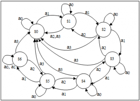
In the proposed MISQ, the finite set of possible environment states S = {s0, s1, s2, s3, s4, s5, s6} (where: s0=15, s1=31, s2=63, s3=127, s4=255, s5=511, s6=1023) includes the different sizes of the contention window corresponding to the 802.11 standard ranging from CWmin= 15 to CWmax= 1023 for each of the two situations (success or collision). The set S of states is represented in the diagram of Figure 1 by the vertices.
Figure 1. Proposition state-transition diagram
Actions are the different decisions based on an action selection method in which, after each transmission attempt regardless of collision or success, a station can either explore environment by choosing an action randomly or following a greedy strategy. The algorithm can transit to a different (s, a) pair and get experience (reward) from it in the random approach. Otherwise, the greedy strategy exploits its so-far gained experience and chooses the action that gives the max Q-value for its current state, presented by Eq. (7).
The set of possible actions in MISQ is A= {stay, increase, decrease, initialize}, presented in Figure 1 by edges a0, a1, a2, a3 respectively, where stay determines the action of staying on the same state in the event of a collision and high queue occupancy rate. The transition increase determines the action to move to the next state in the event of a collision and lower queue occupancy rate. However, decrease defines the action to return to the previous state in the event of successful transmission and lower queue occupancy rate, and initialize means the action to reset to s0 state in the event of a successful transmission and high queue occupancy rate.
Note that a station's generated packets are considered high if Tk, the occupancy queue rate, is greater than 50% and less otherwise, and that each transition in the diagram of Figure 1 is rewarded by a reward Ri (Eq. (14)).
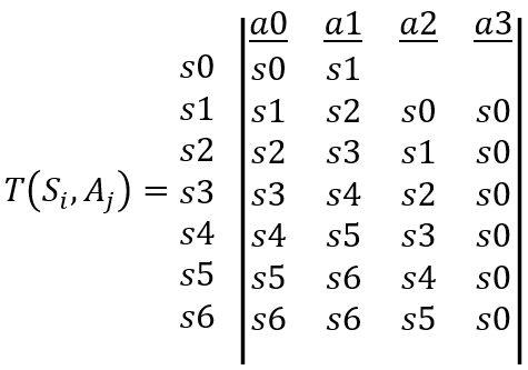
To represent the graph in Figure 1, we use a transition table $T\left(S_{i}, A_{j}\right)$, where $S_{i}, i \in[0,6]$ and $A_{j}, j \in[0,3]$ represent states and actions respectively. The table is given as follows:
4.3 Proposal algorithm
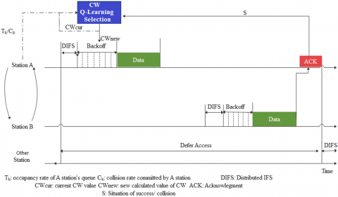
The MISQ algorithm operates essentially as follows: a station transmits a packet and then receives the result S (success or collision) of this transmission, determined by the reception or not of an ACK packet within an acceptable time. The Q-learning agent then adapts the CW value of the station taking into consideration the two parameters Tk and Ck before sending the next packet, and the process is repeated. The operation of the MISQ algorithm is shown in Figure 2.
Algorithm1: CW optimization using MISQ
Global: Q_matrix //to retrieve the previously learned values.
Function Q-learning actions set
if action = stay
CWt+1 = Cwt //No change to CW
else if action = increase and CWt ≠ S6 // S6= CWmax
CWt+1 = Cwt + 1
else if action = decrease and CWt ≠ S0 // S0 = CWmin
CWt+1 =CWt – 1
else
CWt+1 = CWmin
endif
endif
endif
return CWt+1
Function ε –greedy Get-action
Generate p = random_value $\in[0,1]$
if p < ε
Select randomly an action ai $\in$ A
else
select ai* according to the Eq. (7)
endif
return ai
Function CW Q-learning selection
Input: nbpk, nbcolk, Situation // (success or collision)
Output: CW //Optimized Contention windows
Initialize R_matrix, α, γ, ε.
- Evaluate Tk, Ck, the Fitness function and the threshold, Eqns (11), (12), (13) and (15) respectively.
- Calculate the reward function according to equation (14) according to the situation S success or collision.
- Update R_matrix for the couple (s, a) with the reward calculating in the previous point.
- Choose a random action a to explore/exploit (function ε –greedy Get-action)
- Calculate $\Delta \mathrm{Q}(\mathrm{s}, \mathrm{a})$ according to Eq. (10).
- Update the Q_matrix according to Eq. (9) for Q(s, a)
- find the optimal action a* according to Eq. (7).
- Scale CW according to optimal action a* (Function Q-learning actions set).
Return CW.
- Choose a random value of backoff time according to Eq. (16).
Algorithm 1 shows the QL-based contention window selection mechanism (MISQ) that selects the adequate CW value according to acquired experience from its interaction with the environment.
The station s periodically checks the channel if its queue occupancy rate Tk is greater than 0. Once the station has packets to transmit, the backoff time is carried out by selecting the CWt, considering the situation success or collision. The fitness function and the threshold are evaluated, and the reward function is calculated. An action a is chosen by function ε –greedy Get-action and executed to obtain the new state s’ and the reward r. Thus, the Q-matrix function Q(s, a) is updated. Based on the a* value, the maximum Q-Value across all actions in the corresponding learned Q-matrix, the CW is scaled by calling Function Q-learning actions set. Finally, a random value is chosen for the backoff time using the Eq. (16).
Figure 2. Q-learning based MAC protocol
5.1 Simulation setup
In our simulation, we used the network parameters given in Table 1, mostly taken from the 802.11 standard [18]. The simulations are performed using Python [19]. The topology for the simulation is random, and the number of stations varies from 5 to 50, and the stations transmit without RTS / CTS mechanism.
To evaluate the performance of MISQ, we have mainly:
Implement the principle of the algorithm proposed in [14], that we named “QL_BEB” in our figures, and which consists of using two actions in the state space A={0, 1}; where action 0 indicates a decrement of the CW on successful transmission, and action 1 designates an increment of the CW on collision transmission.
Compare the results of the simulations with the classic BEB, as well as the algorithm simulated in 1.
Vary the queue size for each station to 10, 20, or 40 packets, assuming that each station has at least one packet and at most the packet queue size to be transmitted.
Perform many simulations to determine the Q-learning algorithm's parameters to provide good performance to our proposal.
Table 1. Simulation parameters
|
Parameter |
Value |
|
Packet payload |
8,184 bits |
|
MAC Header |
272 bits |
|
PHY Header |
128 bits |
|
Queue Size |
10, 20, 40 |
|
Iteration |
1,500 |
|
Slot time (σ) |
50 µs |
|
DIFS |
128 µs |
|
Max backoff stage (k) |
7 |
|
Retry limit (Rmax) |
4 |
|
CWmin |
15 |
|
CWmax |
1,023 |
5.2 Q-learning parameters
To properly select and evaluate the Q-learning parameters (learning rate α, reduction factor γ, and exploration/exploitation probability epsilon ε), while varying the packet queue size (queue size =10 and, queue size =40), we simulated a network of 25 contended stations while varying the three parameters α, γ and ε: small, medium, and large, to determine the fit values used for the rest of the simulations. We studied the effect of these three parameters on the key performance measure in MANETs which is throughput.
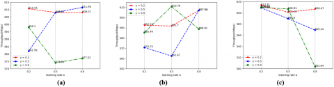
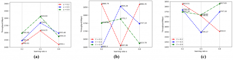
Figure 3 shows the effect of the parameters α, γ and ε on the throughput for a network of 25 stations with a queue size equal to 10, as shown in Figure 3(a), where ε is set to 0.3, α = 0.8, and γ = 0.5 gives the best throughput (611.48Mbps), while a value α = 0.2 degrades the throughput (581.99Mbps) and a value α = 0.5 shows a small change in throughput (608.07Mbps). We also see that a value of γ = 02 gives an almost stable throughput (610.55, 608.07, 608.07 Mbps) whatever the value of α. Figure 3(b) shows that with an average value of α (α = 0.5) and ε (ε = 0.3), it suffices to set γ to its maximum value (γ = 0.9) to have the best throughput (610.78Mbps). However, for α = 0.2 and ε = 0.8, it suffices to set γ to its small value (γ = 0.2) to enhance the throughput (613.31Mbps) as shown in Figure 3(c).
Figure 3. Throughput comparison in network of 25 stations and queue size =10 with (a) ε =0.3 (b) ε = 0.6 and (c) ε =0.8
Figure 4. Throughput comparison in network of 25 stations and queue size =40 with (a) ε =0.3 (b) ε = 0.6 and (c) ε =0.8
Figure 4(a) shows that an average value of α = 0.5, a large value of γ = 0.9, and a small value of ε = 0.3 are effective to give the best throughput (1820.94Mbps). Figure 4(c) shows that where the queue size is equal to 40, with a large value of ε = 0.8, small of γ = 0.2 and small or large values of α (α = 0.2 or α = 0.8) are effective to have a better throughput (1868.74Mbps).
According to the different and multiple simulations performed, we concluded that a combination of a large value of γ, a medium value of α, and a small value of ε cans be significant for different networks with different queue sizes.
5.3 Simulation results
The following parameters are used to measure the performance of the proposal.
5.3.1 Average throughput
The throughput is the ratio of the total amount of data that reaches the receiver from the source and the time taken by the receiver to receive the last packet [20]. It is represented in packets per second or bits per second.
Figure 5 gives the throughput of the MISQ algorithm, in (a) the case where the queue size is equal to 10, (b) the case where the queue size is equal to 20 and (c) the case where the queue size is equal to 40. Compared with the other two algorithms, our proposal gives the best throughput especially from 25 stations regardless of the queue size; this optimization is due to the cumulative rewards learned by the ad hoc network, which is not the case where the number of stations is 5 or 10. The MISQ algorithm achieves better throughput with 20 stations regardless of the queue size.
Indeed, the throughput increases proportionally to the traffic in the network. Beyond 20 stations, the throughput decreases as the number of requests (contended nodes) for access to the channel increases. In terms of throughput, MISQ exceeds BEB and QL_BEB on average by 4.5% and 25.4% respectively. QL_BEB is sensitive to high traffic compared to BEB and MISQ which remains the best.
5.3.2 Average MAC delay access
The average channel access delay for a packet includes the time from the packet being placed at the queue head, until its successful transmission or rejection after the retransmission limit is reached. This time includes the time elapsed in collisions as well as the time spent in the backoff process [6].
Figure 6 shows that the proposed MISQ algorithm gives the least delay or equal to the delay given by BEB, in the case where the queue size equal to 10 (Figure 6(a)) or equal to 20 (Figure 6(b)), on the other hand in Figure 6(c), our algorithm gives the least delay from 45 stations. The channel access delay increases with the density of the network, the more the number of transmissions increases the more collisions there will be, which delays the access to the channel, due to increasing CW. MISQ algorithm gives, on average, the least delay compared to BEB and QL_BEB of 2.64% and 11.17% respectively. For example, with a queue size equal to 20 MISQ algorithm exceeds BEB by 8% and QL_BEB by 22%. It is essential to note that our algorithm MISQ and the simulated one QL_BEB have channel access delays due to the additional learning operations about the environment.
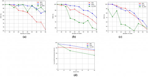
5.3.3 Packet Delivery Ration (PDR)
The PDR represents the number of data packets received by the destination stations per the total number of data packets transmitted by the source station [7]. The PDR is calculated as follows:
$P D R=\frac{\text { Total number of recieved packets }}{\text { Total number of sent packets }}$ (17)
Figure 7 shows the rate of successfully delivered packets. Figure 7(a), where the queue size is equal to 10, shows that MISQ algorithm gives the best PDR that does not drop below 91%, compared to the BEB and QL_BEB having the lowest rate of 66% and 90% respectively. In addition, in the case of a queue size of 20, as shown in Figure 7(b), an obvious visual optimization of the proposed MISQ algorithm, for example, in the case of 50 stations, the rate given by MISQ exceeds by 10% and 20% those given by the BEB and QL_BEB algorithms respectively. In the case where the queue is equal to 50 (Figure 7(c)), the proposal gives the best rate from 30 stations. On average, the proposal provides the best successful transmission rate equal to 90.39%, regardless of the queue size, thus exceeding BEB and QL_BEB by 5.42% and 12.65% respectively, as shown in Figure 7(d).
Figure 5. Network Average throughput for (a): size queue =10, (b) size queue =20, (c) size queue =40
Figure 6. Mac Access Delay for (a): size queue =10, (b) size queue =20, (c) size queue =40
Figure 7. PDR for (a) size queue =10, (b) size queue =20, (c) size queue =40, (d) average successful transmission
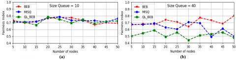
Figure 8. Jain fairness index, (a) size queue=10, (b) size queue= 40
5.3.4 Fairness index
The fairness index between contended stations in Ad Hoc networks is an essential measure of the system. Several measures of equity indices have been proposed in the technical literature, the well-known equation is that of the Jain index [21]. An equity index is a real number that measures the degree to which the resource is fairly or unfairly shared between contended stations.
The fairness index is calculated as follows:
$F I=\frac{\left(\sum_{i=1}^{N} x_{i}\right)^{2}}{N \times \sum_{i=1}^{N} x_{i}{ }^{2}}$ (18)
where, xi is the access portion of station i among N contended stations.
The fairness index of the three algorithms is almost identical in the case where the queue size is equal to 10 (Figure 8(a)), with an almost stable index varying between 70% to 78% for MISQ, the index of BEB algorithm varies between 69% to 78%, while it varies between 66% and 78% for the QL_BEB algorithm. On the other hand, in the case where the size queue is equal to 40 (Figure 8(b)), BEB algorithm gives the best average index equal to 70% compared to those of MISQ and QL_BEB algorithms which are 63% and 52% respectively. This dropping in the index of MISQ is due to the favor given to the stations which have a high occupancy rate regardless of the situation (success or collision).
In this paper, we present an algorithm that exploits the deep reinforcement learning principles to learn the correct CW parameters for the 802.11 standard to optimize the contention window. Motivated by the characteristics of deep reinforcement learning (DRL) in wireless networks, we use one of its techniques: Q-learning, as a channel resource allocation paradigm in the MAC layer. The proposal, named MISQ, focuses on optimizing the contention window CW by considering the occupancy rate of the packets queue to be transmitted and the collisions made by each station after each successful or collision transmission. These are ensured by preserving other network parameters such as throughput and channel access time. The results of the simulations show that the proposed algorithm based on Q-learning optimizes BEB performance in terms of PDR, throughput, and channel access time, especially when the queue size is less than or equal to 20 regardless the number of stations (10 to 50).
The formulation of a mathematical model for the proposed MISQ mechanism will be the objective of future work.
[1] Xu, S., Saadawi, T. (2001). Does the IEEE 802.11 MAC protocol work well in multihop wireless ad hoc networks? IEEE Communications Magazine, 39(6): 130-137. https://doi.org/10.1109/35.925681
[2] Al-Hubaishi, M., Abdullah, T., Alsaqour, R., Berqia, A. (2012). EBEB algorithm to improve quality of service on wireless ad-hoc networks. Research Journal of Applied Sciences, Engineering and Technology, 4(7): 807-812.
[3] Challita, U., Dong, L., Saad, W. (2017). Proactive resource management in LTE-U systems: A deep learning perspective. [Online]. Available: https://arxiv.org/abs/1702.07031
[4] Ali, R., Zikria, Y.B., Kim, B.S., Kim, S.W. (2020). Deep reinforcement learning paradigm for dense wireless networks in smart cities. In Smart Cities Performability, Cognition, & Security, Springer, Cham, pp. 43-70. https://doi.org/10.1007/978-3-030-14718-1_3
[5] Moon, J., Lim, Y. (2017). A reinforcement learning approach to access management in wireless cellular networks. Wireless Communications and Mobile Computing. https://doi.org/10.1155/2017/6474768
[6] Williams, B., Camp, T. (2002). Comparison of broadcasting techniques for mobile ad hoc networks. In Proceedings of the 3rd ACM International Symposium on Mobile Ad Hoc Networking & Computing, pp. 194-205. https://doi.org/10.1145/513800.513825
[7] Tseng, Y.C., Ni, S.Y., Chen, Y.S., Sheu, J.P. (2002). The broadcast storm problem in a mobile ad hoc network. Wireless Networks, 8(2-3): 153-167. https://doi.org/10.1023/A:1013763825347
[8] Natkaniec, M., Pach, A.R. (2000). An analysis of the backoff mechanism used in IEEE 802.11 networks. In Proceedings ISCC 2000. Fifth IEEE Symposium on Computers and Communications, pp. 444-449. https://doi.org/10.1109/ISCC.2000.860678
[9] Balador, A., Movaghar, A., Jabbehdari, S., Kanellopoulos, D. (2012). A novel contention window control scheme for IEEE 802.11 WLANs. IETE Technical Review, 29(3): 202-212. https://doi.org/10.4103/0256-4602.98862
[10] Yassein, M.B., Alomari, M.A., Mavromoustakis, C.X. (2012). Optimized pessimistic Fibonacci back-off algorithm (PFB). International Journal of Advanced Computer Science and Applications, 3(9). https://doi.org/10.14569/IJACSA.2012.030939
[11] Deng, J., Varshney, P.K., Haas, Z.J. (2004). A new backoff algorithm for the IEEE 802.11 distributed coordination function. Electrical Engineering and Computer Science. Paper, 85. http://surface.syr.edu/eecs/85
[12] Shahin, N., Ali, R., Kim, S.W., Kim, Y.T. (2019). Cognitive backoff mechanism for IEEE802. 11ax high-efficiency WLANs. Journal of Communications and Networks, 21(2): 158-167. https://doi.org/10.1109/JCN.2019.000022
[13] Wydmański, W., Szott, S. (2020). Contention window optimization in IEEE 802.11 ax networks with deep reinforcement learning. arXiv preprint https://arxiv.org/abs/2003.01492
[14] Ali, R., Shahin, N., Zikria, Y. B., Kim, B. S., Kim, S.W. (2018). Deep reinforcement learning paradigm for performance optimization of channel observation-based MAC protocols in dense WLANs. IEEE Access, 7: 3500-3511. https://doi.org/10.1109/ACCESS.2018.2886216
[15] Sutton, R.S., Barto, A.G. (2018). Reinforcement learning: An introduction. MIT press. [Online]. Available: http://www.incompleteideas.net/book/RLbook2018trimmed.pdf.
[16] Watkins, C.J.C.H. (1989). Learning from delayed rewards. Thesis submitted for Ph.D.
[17] Alpaydm, E. (2014). Introduction to Machine Learning, 3rd ed. Cambridge, MA, USA: MIT Press.
[18] IEEE Standard for Information Technology-Telecommunications and information exchange between systems Local and metropolitan area networks-Specific requirements - Part 11: Wireless LAN Medium Access Control (MAC) and Physical Layer (PHY) Specifications. (2016). In IEEE Std 802.11-2016 (Revision of IEEE Std 802.11-2012), pp. 1-3534. https://doi.org/10.1109/IEEESTD.2016.7786995
[19] python version 3.7. https://www.python.org/downloads/release/python-370/.
[20] Peng, X., Jiang, L., Xu, G. (2007). Performance analysis of hybrid backoff algorithm of wireless LAN. In 2007 International Conference on Wireless Communications, Networking and Mobile Computing, pp. 1853-1856. https://doi.org/10.1109/WICOM.2007.464
[21] Jain, R.K., Chiu, D.M.W., Hawe, W.R. (1984). A quantitative measure of fairness and discrimination. Eastern Research Laboratory, Digital Equipment Corporation, Hudson, MA.