Mahendra Pratap Yadav* | Gaurav Raj | Harishchandra A. Akarte | Dharmendra Kumar Yadav
© 2020 IIETA. This article is published by IIETA and is licensed under the CC BY 4.0 license (http://creativecommons.org/licenses/by/4.0/).
OPEN ACCESS
Cloud computing is a paradigm to provide services to end-users through the Internet. The availability of services to end-users is dependent on various factors such as the availability of computing resources as well as the number of users to access those services. To manage the real-time fluctuating workload cloud providers use elasticity mechanisms. Elasticity is one of the important characteristics of cloud computing that dynamically allocates computing resources to manage the fluctuating workload. The failure of allocation/de-allocation of computing resources at the right moment leads to SLA violation, degradation of services performance, maximum power consumption, minimum throughput, and maximum response time. To address these challenges, we have proposed a hybrid approach to perform horizontal elasticity. The proposed approach uses both reactive and proactive approaches for provisioning/de-provisioning of computing resources. The simulation results of the proposed model show that performance of system has improved in terms of CPU utilization, response time, and throughput.
cloud computing, elasticity, auto-scaling, machine learning, ARIMA, support vector machine
In the current era, cloud is an emerging technology that provides on-demand resources for varying requirements on the basis of a lease. There are various cloud platforms and virtual data-centers, which provide elasticity of services in order to handle the rapidly changing workload [1]. Elasticity is the ability of a system to increase /decrease resources to adopt the load variation in real-time. It is a dynamic property of cloud computing. There are two advantages of service elasticity, first is Quality of Service (QoS) which is achieved by optimizing certain parameters such as response time, CPU load, numbers of requests handled in a second, etc. There is an agreement between cloud resource providers and clients to ensure QoS using Service Level Agreements (SLAs). The second advantage is that it reduces the overall power consumption by preventing the system from over-provisioning of resources. Over provisioning means, more resources have been allocated than required to handle peak loads. Elasticity mainly involves scalability and efficiency. Efficiency is about the percentage of utilization of available computing resources while scaling is performed. The lower the amount of resources needed the better is the efficiency. Scalability is the property of a machine, which enables it to handle the more workload by adding more resources.
Cloud providers use a virtualization-based approach in order to host their services. Virtualization [1, 2] refers to the act of creating a virtual resource, including computer hardware platforms, storage devices, and computer network resources. Virtualization can be implemented with the help of hypervisors and containers [3]. In comparison to hypervisors, containers are lightweight software, which have quick start or stop time and less overhead than virtual machines. Containers allow a software developer to pack up an application with all of its requirements, such as libraries and other dependencies, and it can be shipped out as one package [2, 3]. Auto scaling can be performed in two ways, which are reactive and proactive approaches [4]. In reactive approach, one or more threshold(s) can be used which need to be optimized such as response time, CPU load, memory usage, etc. After a certain interval, we find the resources exceeding this threshold and based on that, resources can be increased or decreased. On the other hand, in proactive scaling, we predict the workload of upcoming time interval by applying some machine learning or deep learning algorithms. After the prediction of workload, we find the amount of resources needed to manage the load. While using proactive approaches care should be taken for not performing premature scaling operation. Premature scaling means, just after scaling down, flood of requests arrives and we have to scale up the resources again [5]. Therefore, premature scaling will add overhead and will not be effective from cloud provider’s point of view.
Auto-scaling can be more efficient if we use combination of reactive and proactive approaches [4, 6]. Various proactive approaches can be used to analyze the time-series data such as AR (Auto Regressive), MA (Moving Average), ARMA (Auto Regressive Moving Average), ARIMA (Auto-Regressive Integrated Moving Average), etc. in order to predict the future workload [4, 7]. The future workload can be transferred over various machines through load balancer. The load balancer uses different load balancing algorithms to distribute the workload dynamically and uniformly across all the available nodes. This improves the overall system performance. Cloud load balancing is defined as the method of splitting workloads and computing properties in a cloud-computing environment [8, 9].
In this article, we have discussed a hybrid algorithm that uses a reactive model (threshold-based policy) and time series forecasting based proactive model for the provisioning and de-provisioning of computing resources based on workload in real time. The reactive approach is used for scaling out the running containers when the workload increases and proactive approach (Support Vector Regression (SVR)) for scaling in the containers when the workload decreases. The experimental results of proposed hybrid approach are compared with time series forecasting models (ARIMA, and SARIMA). Based on comparisons, we have found that the performance of proposed hybrid approach is better than other two models in terms of horizontal scaling, average CPU utilization and response time.
The rest of paper is organized as follows: In section 2, motivation for the proposed work has been described. In section 3, background and related technology have been given. Section 4 presents the literature review for the work. In section 5 solution of the problem has been proposed. In section 6 experimental setup and result analysis have been done and the last section (i.e. Section 7) concludes the work along with future directions.
We have observed in many cases that the resources on the cloud system have been underutilized and some requests from the users are dropped. However, the request would have been serviced, if there had been scaling of resources based on the demand of the users. In addition, it would be very tedious to scale the resources manually hence; we thought to scale up the resources automatically through a scaling algorithm. We have used horizontal scaling to handle workload with the help of a load balancer. We have tried to search many metrics regarding running containers and requests that are available to us that can be potentially used to tell the state of the system. But, we found that the response time produced by logs of load balancer could be a very good metric to gain insight into the current load on the system. The reactive model is used basically to quickly scale-out in case of increasing workload. The proactive model is primarily used to scale-in since it uses past data to forecast future workload. Hence, we decided to scale horizontally according to the response time of live requests to the web server.
3.1 Docker
Docker is an open software, which provides centralized platform to execute an application. Docker wraps software components into a complete standardized unit, which contains everything required to run it i.e. runtime environment, tools or libraries [10]. It guarantees that the software will always run as expected. It provides the facility to run an application in an isolated environment, which is called container. We can run multiple containers simultaneously on a given host. It is lightweight as compared to hypervisors, so it starts instantly and uses less RAM. Docker is secure by default because each container is isolated from one another. Docker works as a client-server architecture. The Docker-daemon (server) receives the commands from the Docker client through CLI or rest APIs. Docker client and server can be present on the same host machine or different hosts.
3.2 Docker swarm
A Docker swarm contains a group of systems, which are running Docker and joined to make a cluster. It is a tool for container Orchestration. Docker swarm is used to do health check of every running container, ensure containers are upon every system, scaling in or out the containers depending on the upcoming load, and adding updates in the containers. These above tasks are difficult to perform manually. Orchestration means managing and controlling multiple Docker containers as a single service. Docker Swarm, Kubernetes and Apache Mesos are the tools available for orchestration. Containers in a swarm are called nodes. Some nodes are made manager and some are made workers. The manager node has total control on the swarm created. The manager node assigns units of work called tasks to worker nodes. We use Docker swarm to easily use utilities for scaling up and down as the algorithm decides the required number of containers [10].
3.3 HAProxy
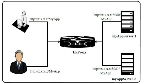
HAProxy stands for High Availability Proxy, which is used as a TCP/HTTP load balancer and provides proxying solution [11, 12]. It acts as a TCP proxy that can accept a TCP connection from a listening socket and then connect to a server which allows the traffic to flow in both directions. It also acts as an HTTP reverse proxy, which receives HTTP requests on a listening TCP socket and then passes these requests to servers using different connections. Figure 1 shows the basic architecture of HAProxy load balancer.
Figure 1. HAProxy configuration
In this article, HAProxy acts as a server load balancer, which is used for balancing the load of TCP connections and HTTP requests. It spreads various requests across multiple servers in order to optimize resource usage, maximize throughput, avoid overloading of any server and minimize response time. When the Tsung Benchmarking tool generates the workload it gets transferred over the load balancer. For this, we have used the HAProxy load balancer. The load balancer transfers the incoming request over the server. The load balancer stores all the logs of incoming request. This log data will be used in proactive approach to perform the scale in operation. There are various algorithms available in HAProxy load balancer namely: Round robin, least connection, and source IP for balancing the load.
By default, HA Proxy balances the requests in a round robin manner between the containers hosting the server. It only requires the HAProxy executable and a configuration file to run. It is highly recommended to have a rsyslog daemon for logging and the configuration files are parsed before starting in order to bind all the listening sockets. Once HA Proxy is started, it processes the incoming connections, periodically checks the server’s status and exchanges information with other HAProxy nodes. The processing of incoming connections is the most complex task as it depends upon the configuration possibilities and the various steps are as follows [11]:
3.4 Tsung benchmarking tool
We have used Tsung [13] for load testing of the system. The programming language used by Tsung, is Erlang. It is used for performance testing of a website, which is important for the success of any website. It is also an important tool because certain business sites have suffered serious downtimes when they have a large number of visitors. If they use this tool before their website or application deployment then they can check the tolerance of their websites for large number of loads. Tsung benchmarking tool has the following features:
Tsung Benchmarking Tool has been used to generate the load over the server. The tolerance of the proposed approach is that the system does not go under load or overload. If it does, they demand extra computing resources to manage the workload. The additional computing resource is namely CPU. The resource allocation or de-allocation is depended on the predefined upper and lower threshold values. The upper and lower predefined threshold values of computing resources are 85 percent and 20 percent, respectively.
In this section, work related to the recourse provisioning and de-provisioning to manage the fluctuating workload for time series data has been studied. Along with time series data forecasting methods, many researchers have proposed an auto-scaling mechanism based on many different strategies, namely threshold-based or rule-based, control theory, reinforcement learning, and queuing theory [6, 8, 14].
Al-Dhuraibi et al. [14] have presented a literature survey on elasticity in cloud computing. The authors present the survey for VMs and container-based elasticity, which has highlighted the basic taxonomy of elasticity. This survey is divided into three segments; the first define elasticity and related concepts such as scalability and efficiency. They presented the extended classification of elasticity based on the configuration, scope, purpose, mode, policy, method, provider, and architecture, which will be used to obtain different aspects. The third presented the existing technology that is related to the container. The authors also discussed the open issues and research challenges about container elasticity. The authors pointed different topics such as interoperability, granularity, resource availability, a hybrid solution, start-up time, threshold definition, prediction estimation error, an optimal trade-off between the user’s requirement and provider’s interests, a unified platform for elastic application and evaluation methodology. They also presented the research challenges about container-based elasticity such as monitoring containers, container-based elasticity, combined elasticity between VMs and containers.
Al-Dhuraibi et al. [15] presented a reactive approach that is rule-based. This approach is used for vertical elasticity of container with the help of ELASTICDOCKER. The ELASTICDOCKER is an auto-scaler that is used to adjust the container computing resources like memory and virtual CPU cores based on workloads. The upper and lower threshold values of a container are adjusted according to different experimentation values, and then one of them, which has the least response time, is chosen. The authors have allocated/de-allocated the computing resources (memory and CPU) to a container in a fixed manner. For example, when container memory utilization has a value greater than the upper bound of hits, then 256 Mb of memory is added to the container by the auto-scaler. On the other hand, when the container memory utilization is lower than the threshold, the auto-scaler will decrease 128 Mb of memory. For de-provisioning, an auto-scaling step is used so that there is no unexpected interruption in the application's functionality when it is running. In addition, the authors also do a live process migration from a hosted machine to another machine when the resizing of a container is not possible on the host machine.
Al-Dhuraibi et al. [16] have presented to coordinate the container as well as virtual machine for vertical elasticity. Authors have performed an auto-scaling mechanism for containerized applications so that their computing resources can be adjusted at both the container and VM levels with an elastic controller's help according to the workload. This controller directly modifies the container file system, namely cgroup to execute the scaling mechanism (scaling up/down). This scaling mechanism is executed based on the average utilization of CPU or memory over a fixed interval of time and compared it with its upper/ lower thresholds (70% 90%) value. When the value after calculation reaches the threshold or the logical conditions are met, the value of resources increases or decreases by the controller using the values based on a predefined rule. For example, suppose if the average memory consumption of a container is greater than the upper threshold for the last 16 seconds, memory size is increased to 256 MB by the controller. It waits 10 seconds before accomplishing the next scaling action. The proposed elasticity controller for container vertical make it up to 18.34% and vertical elasticity controller for VM makes it up to 70%. The proposed strategy also outperforms horizontal elasticity by 39.6%.
Rule-based auto-scaling mechanisms are implemented in the reactive approach. Different cloud organizations and their platforms (such as Amazon EC2, Microsoft Azure, RightScale, Docker, Open Stack, and OpenNebula [17]) use the reactive approach to provide the computing resources to end-users. Cloud providers define their scaling policies based on different computing resource metrics to perform scale-up or down a machine's resources. In the rule-based scaling approach, the trigger action can be performed on a threshold value, either the upper threshold or lower threshold value. The trigger action can be performed when the selected metric is over (or under) the specific threshold for a certain time interval period. The trigger action can request auto-scalar to add or remove a certain amount of computing resources from the physical infrastructure to a machine. Some academician has worked specific improvements for threshold-based technique, for example, Hasan et al. [18] have implemented their auto-scaling policies by considering the four threshold values. If the auto-scaling strategy uses two thresholds value, the auto-scaling perform finer decision. Besides the rule-based auto-scaling mechanism, many researchers have proposed an auto-scaling mechanism with control theory concepts. They have been implemented through a controller. The controller is responsible for maintaining the system performance at a specific level with a control input. Maximum control-based systems use the reactive mechanism.
DoCloud [19] provides an auto-scaling platform for an elastic service. It finds out the number of containers required according to the dynamic workload. It uses both reactive and proactive approaches for auto-scaling, where the reactive approach is used for scaling-out, and a proactive approach is used for scaling-in the number of containers. In the reactive approach, the threshold-based method is done by comparing the CPU utilization of each container with a threshold value, and in the proactive approach, ARMA (Auto Regressive Moving Average) model is used for time series forecasting of the workload and then convert it into the required number of containers. It uses a hybrid approach, i.e., reactive as well as proactive approaches, to avoid a premature scale-in operation, which causes oscillations in the number of containers. The threshold-based mechanism is a reactive auto-scaling algorithm that enables users to define scaling up and scaling down policies or rules based on different metrics. These rules are defined as the lower and upper threshold for selected metrics.
There are several auto-scaling mechanism proposals based on the concept of control theory [20]. Most control systems are based on reactive mechanisms. They usually implement a controller that is responsible for maintaining the output of the system. A controller has been implemented for maintaining the system output at the desired level. The feedback controller system [18, 21, 22] has the input at the desired level by provisioning or de-provisioning resources. Another work for auto elasticity was HPA (Horizontal Pod Autoscaler) [23], which scales the number of containers that serve a given application when the average CPU consumption by containers is greater than the CPU average threshold value. This auto-scaler is implemented as a control loop where it periodically queries the CPU utilization to create a sufficient number of containers (pods).
Container Resource Utilization Prediction Algorithm (CRUPA) [24] is also another auto-scaling method. This method used the ARIMA model for predicting the CPU utilization and correspondingly to perform scaling of the resources. It performs better than a threshold-based approach, but the identification of parameters is a time-consuming task. Also, it is not efficient to handle the oscillations in the workload. In this paper, we have proposed an algorithm for load balancing, i.e., Hybrid algorithm which uses both reactive as well as proactive approach.
The proposed approach is different from the threshold-based approach because our algorithm can efficiently handle the oscillation mitigation (due to the use of a proactive approach also), but this approach can cause sudden provisioning or de-provisioning of the resources based on workload. Our proposal is different from DoCloud because DoCloud uses only the ARMA model for predicting the workload, but we have used ARIMA and SVR models also and then presented the comparison between the scaling results, response rates, and CPU utilization. Our proposal is different from the control system approaches because they are also reactive approaches, and hence the problem of oscillation mitigation will occur there. Our proposal is different from HPA because HPA performs CPU consumption measurements, and our algorithm also uses the CPU consumption. Still, along with this, it also uses a predictive method for scaling, which is not available in HPA. CRUPA performs CPU utilization prediction, but our algorithm performs workload prediction, and CRUPA performs sudden scaling of resources based on a proactive approach but our algorithm uses a reactive approach for scale-out and proactive approach for scale-in only when the system becomes stable.
5.1 Time series forecasting
Time Series [7, 25] data are experimental data observed at various point in time. For example, any product like soap, clothes, etc. has sales per day. Time Series data has many characteristics like seasonality, trend and noise. Forecasting is simply predicting the future data based on current and past data. ARIMA (Auto Regressive Integrated Moving Average) is one of the methods, which can be used for the forecasting. In an ARIMA model, three parameters that are used to help model the major aspects of a times series [25]: Seasonality(p), trend(d), and noise(q).
For the simulation of ARIMA model, three parameters, namely seasonality (p), trend (d), and noise (q) has been used. We have to fit the ARIMA (0, 1, 1) model. This sets the lag value to 0 for auto-regression; the ARIMA model's difference order is 1, which makes the time series stationary, and uses a moving average model of 1.
The mathematical equation is used by ARIMA model is [4]:
y(t) = µ+φ1yt−1+......+φpyt−p−θ1et−1−......−θqet−q (1)
where, µ is a constant, φ terms are the lagged values of y (AR term), and θ terms are lagged values of error (MA term). There is also an enhancement of ARIMA model, which is dependent on the seasonality of the data, that is known as Seasonal ARIMA (SARIMA). Seasonality means the changes in the data that forms a regular pattern and keeps repeating itself after fixed time interval. SARIMA incorporates both seasonal and non-seasonal factors like a multiplicative model. A seasonal ARIMA model is formed by including additional seasonal terms in the ARIMA […]. The seasonal part of the model consists of very similar words to the model's non-seasonal components, but they involve backshifts of the seasonal period. To configure SARIMA, it requires different hyper parameters for both the series's trend and seasonal elements [26, 27]. For the simulation we have used SARIMA with order (1, 1, 1) and seasonal order (0, 0, 0, 12).
Another important time series-forecasting model is SVR (Support Vector Regression). Support Vector Regression [4, 28] is a regression model, which uses same principles as SVM (Support Vector Machine). Following are the important parameters of SVR:
Consider two boundary lines (Decision Boundary Lines) are ‘a’ distance from hyper plane. Therefore, these are lines that we draw at a distance ‘+ɛ’ and ‘−ɛ’ from the hyper plane. Assuming that the equation of hyper plane is as follow:
Y = wx + b (2)
Then the equation of decision boundary become:
wx + b = ɛ (3)
wx + b = − ɛ (4)
Thus, any hyper plane that satisfies our SVR should satisfy:
ɛ −< Y − wx − b < + ɛ (5)
Our main aim here is to decide a decision boundary at ‘ɛ’ distance from the original hyper plane such that data points closest to the hyper plane or the support vectors are within that boundary line. Hence, we are going to take only those points that are within the decision boundary and have the least error rate, or are within the Margin of Tolerance. This gives us a better fitting model.
5.2 Proposed scaling models
(1) Reactive Model: This model is used to scale-out the number of containers. Since the load increases rapidly, we need to increase quickly the instances of our webserver to manage the fluctuating workload. Therefore, the reactive approach is best for rapidly handling the huge load. Developers set an upper threshold for some resource utilization; the system collects the resource utilization data in every container at a certain time interval. If some of the containers’ resource utilization exceeds the given upper threshold, new containers are spawned, more containers will be started and added to handle the varying load. The Reactive Model Scaling [22] algorithm (i.e., Algorithm 1) is as follows:
|
Algorithm 1: Reactive Model Scaling |
|
Input: Initial running containers, i.e., n_current Output: Required number of containers
|
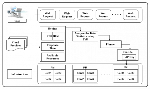
(2) Proactive Model: Proactive models are mainly used to scale-in the number of containers. We have used ARIMA, SARIMA, and SVR as our proactive algorithms. For ARIMA and SRIMA, we used the grid search to find the optimal set of parameters that yield our model's best performance. We used the minimum AIC (Akaike Information Criteria) value to select parameters for our model. We used the Radial Basis Function (RBF) kernel to calculate the workload for SVR. The hybrid algorithm is used either after a long time or when the system is stable or safe to reduce the number of containers. It runs after a short period of ∆(T) to forecast the future load. This predicted load is then converted to the required number of containers. Figure 2 shows the working procedure of the MAPE architecture that can be used for workload prediction, and based on that hybrid approach, it finds out how many containers are required to manage the fluctuating workload.
5.3 Hybrid scaling algorithm
Reactive and Proactive both models are used simultaneously to perform the horizontal scaling (i.e., Algorithm 2). As scale-out should be quick enough, since the load is changing rapidly, we use the reactive model for this purpose. We use docker API in python to scale in and out web server services. The scale-in should not be premature; otherwise, it may cause oscillations in the number of containers if clients' requests are increased quickly just after scale-in occurs. Scale-in should only occur when the web application does not need the containers any more in the near future. In our algorithm, only during the following continuous k periods, the numbers of containers predicted by the proactive model are all below current running containers, and then some containers will be stopped. Algorithm 2 shows the hybrid model scaling approach that can perform the horizontal elasticity.
Figure 2. MAPE working procedure
|
Algorithm 2: Hybrid Model Scaling |
|
Input: Initial running containers, i.e., n_current and delay for scale in, i.e., max_scaling_period Output: Required number of containers
|
In this section, we have discussed all the necessary steps that are used to implement proposed scenario.
6.1 Create a Docker compose file
Docker composes files and commands are used to deploy the services on the swarm and specify the initial configuration of the available containers:
docker stack deploy -c [DOCKER COMPOSE FILE]
STACK_NAME
In this Docker-compose file, we specify the images used by services. We specify the replicas for each service, i.e., initial no. of containers, port mappings, and resource limits for CPU and memory. Since we required one HTTP server, so for that purpose, we used HAProxy, and hence we need to create a container with HAProxy that would listen to port 3000 and balance the load for the request to different web server containers listening on port 80. In order to create these containers, we have created a Docker-compose file, with the help of that we have created two services:
6.2 Create a docker swarm
Docker swarm is used to manage the containers in an efficient manner in order to increase the throughput. The following command is used to initialize the swarm
docker swarm init
The network, all the services and all the containers are called stack. To create our web stack using node server containers and HAProxy containers, we used Docker stack command, but we want to point to the stack of our docker-compose.yml file, so it will build the stack according to our plan there. We can do it by writing the following command:
Docker stack deploy --compose-file= docker- compose.yml
We used the deploy command to deploy a new stack. It can also be used to update an existing stack. When we hit http://localhost:3000/, then we will be getting the container id in the response.
6.3 Generating load using Tsung benchmarking tool
We have used Tsung in order to generate the workload. Tsung gives us flexibility to generate the variable and constant load, which helps us to improve our prediction. And it helps us to visualize the different variations in load. For the generation of the load, we define a load progression step in XML file. The format is something like:
<load>
<arrivalphase phase="1" duration=
"10"unit="minute">
<users interarrival="2" unit=
"second"></users>
</arrivalphase>
</load>
With this setup, during the 10 minutes of the test, a new user will be created in every 2 seconds. It is up to us to add any number of arrival phases, as we want. We can also add maximum number of users, which can be generated in one arrival phase. Tsung is also used to produce log files, reports and graphs for real time analysis. It produces these analytic on port 8091.
6.4 Plotting of the results
For the plotting of the results, we have used Gnu plot, which is a command-line driven graphing utility for Linux. Here, we are plotting the number of containers corresponding to the workload versus time graph.
set style line 1 lc rgb ’#0060ad’ lt 1
lw 2 pt 7 ps 1.5
plot ’plotting_data.dat’ with
linespoints ls 1
6.5 Result analysis
To explain the working procedure, we have created two different scenarios of load using Tsung. The two scenarios are completely opposite of each other and show how our algorithm is able to adapt these different use cases.
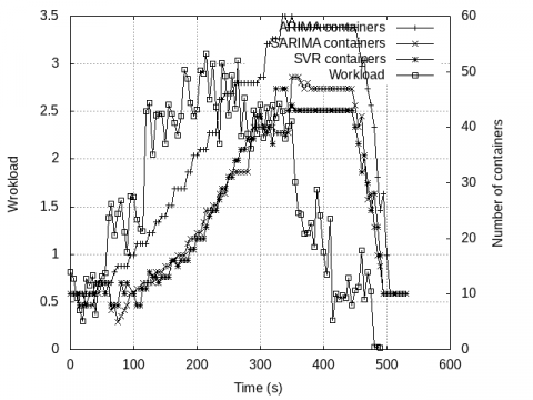
In first scenario (Figure 3), the number of containers varies quickly with respect to changing load. As load increases, the reactive model is quick to scale-out. In the duration of stable load, numbers of containers remain constant. Then as the load drops, our proactive model reduces the number of containers once the load keeps decreasing. In the simulation, we have considered one parameter such as CPU load. The proposed approach performs horizontal elasticity. In the horizontal elasticity, when the computing resource utilization reaches up to a predefined threshold, the auto-scaler performs the trigger action and creates a new machine instance. When we go for vertical elasticity, then we will use the single parameter. In vertical elasticity, we will increase or decrease the single parameter based on the utilization.
Figure 3. Number of Containers v/s Workload for Scenario 1
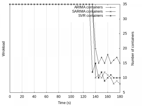
Figure 4. Number of Containers v/s Workload for Scenario 2
In second scenario (Figure 4), even if the variation of load is high, our algorithm does not hastily decrease the number of containers until the load is stable. The number of the container decreases in the proactive mode. The proactive approach is used to predict the number of containers still needed in the future to manage the workload. When the algorithm requests to execute the scale-out command, the auto-scaler waits 10 seconds before executing it. In this time interval if the workload suddenly increases, it protects the system from going into an overloaded state. It stays 10 seconds, which avoids system failure, so it does not waste computing resources. This ensures better QoS and makes it less sensitive to flash crowds.
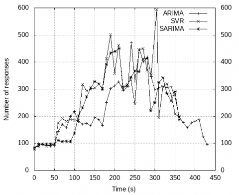
We have also shown the comparison between different predictive models that we have used like ARIMA, SARIMA and SVR. From Figure 3, we can observe that the maximum number of containers required is least in SVR and it can predict the decrements in workload much efficiently. In Figure 5, we have also compared the number of responses fulfilled per second when using three different predictive models and here we can observe that the response rate of SVR is better than other two models, i.e., SVR fulfill more requests per second and SARIMA also performs quite good in terms of requests fulfillment.
Figure 5. Comparison of Response rate
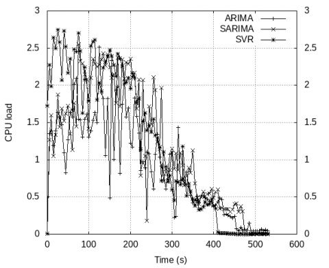
Figure 6. Comparison of CPU utilization
In Figure 6, we have also compared the average CPU utilization of all the running containers using these three models and observed that the CPU utilization is better in SVR followed by SARIMA and lastly ARIMA model for prediction in workload.
In Figure 6, the simulation has been done through workload generated tool, namely Tsung. The load varies with the number of increases or decreases in hits. The Tsuing can generate 5000 requests/second. With the different time interval and number of hits, the number of containers may increase or decrease in the simulation. The simulation has been done in both the minimum and maximum load to check the system performance and increase/decrease the number of containers. The proposed approach uses the reactive approach to increase the number of containers when the workloads increase, and a proactive approach when the number of containers decreases.
Table 1. Number of Containers corresponding to Workload
|
Sr. No. |
Timer |
Workload |
Hybrid using ARIMA model |
Hybrid using SARIMA model |
Hybrid using SVR model |
|
1 |
0 |
0.815 |
10 |
10 |
10 |
|
2 |
10 |
0.5425 |
10 |
10 |
10 |
|
3 |
50 |
0.77 |
12 |
12 |
12 |
|
4 |
100 |
1.5975 |
17 |
10 |
10 |
|
5 |
150 |
2.16 |
24 |
15 |
13 |
|
6 |
200 |
2.5225 |
35 |
21 |
20 |
|
7 |
250 |
2.46 |
46 |
31 |
31 |
|
8 |
300 |
2.5725 |
49 |
40 |
42 |
In Table 1, we have shown the required number of containers corresponding to changing workload for all three models, i.e., ARIMA, SARIMA and SVR, which we have used in our hybrid algorithm.
The proposed strategy explores the use of a hybrid approach using both reactive and proactive models for horizontal scaling (e.g., number of containers) to manage the fluctuating workload. The reactive model is used basically to quickly scale-out in case of increasing workload. The proactive model is primarily used to scale-in since it uses past data to forecast future workload. Even with a high load variation, this algorithm does not hastily decrease the number of containers until the load becomes stable. The proposed approach gets the best of both reactive and proactive scaling and tries to eliminate any limitations if these approaches are applied exclusively. The experimental results also show that it offers good efficiency and scalability. In the future, we can use this model for hybrid scaling, where horizontal and vertical scaling is done together to make it more efficient. Here, we consider only one variable for the forecasting; for better results, we can use other variables like memory, users, CPU, etc. We can also use other sophisticated algorithms like TOPSIS, PID, etc, for reactive and proactive scaling and compare it to our current results.
This research was supported/partially supported by [Visvesvaraya PhD scheme for Electronics and IT, Ministry of Electronics and Information Technology, Government of India]. We thank our colleagues from [Motilal Nehru National Institute of Technology Allahabad, Prayagraj, India] who provided insight and expertise that greatly assisted the research, although they may not agree with all of the interpretations/conclusions of this paper.
[1] Zhang, Q., Cheng, L., Boutaba, R. (2010). Cloud computing: state-of-the-art and research challenges. Journal of Internet Services and Applications, 1(1): 7-18. https://doi.org/10.1007/s13174-010-0007-6
[2] Smith, J., Nair, R. (2005). Virtual Machines: Versatile Platforms for Systems and Processes. Elsevier. https://doi.org/10.1016/B978-1-55860-910-5.X5000-9
[3] Seo, K.T., Hwang, H.S., Moon, I.Y., Kwon, O.Y., Kim, B.J. (2014). Performance comparison analysis of Linux container and virtual machine for building cloud. Advanced Science and Technology Letters, 66(105-111). https:// doi.org/10.14257/ASTL.2014.66.25
[4] Moreno-Vozmediano, R., Montero, R.S., Huedo, E., Llorente, I.M. (2019). Efficient resource provisioning for elastic Cloud services based on machine learning techniques. Journal of Cloud Computing, 8(1): 5. https://doi.org/10.1186/s13677-019-0128-9
[5] Jiang, J., Lu, J., Zhang, G., Long, G. (2013). Optimal cloud resource auto-scaling for web applications. In 2013 13th IEEE/ACM International Symposium on Cluster, Cloud, and Grid Computing, Delft, Netherlands, pp. 58-65. https://doi.org/10.1109/CCGrid.2013.73
[6] Roy, N., Dubey, A., Gokhale, A. (2011). Efficient autoscaling in the cloud using predictive models for workload forecasting. 2011 IEEE 4th International Conference on Cloud Computing, Washington, DC, USA. https://doi.org/10.1109/CLOUD.2011.42
[7] Messias, V.R., Estrella, J.C., Ehlers, R., Santana, M.J., Santana, R.C., Reiff-Marganiec, S. (2016). Combining time series prediction models using genetic algorithm to autoscaling web applications hosted in the cloud infrastructure. Neural Computing and Applications, 27(8): 2383-2406. https://doi.org/10.1007/s00521-015-2133-3
[8] Cocaña-Fernández, A., Sánchez, L., Ranilla, J. (2016). Leveraging a predictive model of the workload for intelligent slot allocation schemes in energy-efficient HPC clusters. Engineering Applications of Artificial Intelligence, 48: 95-105. https://doi.org/10.1016/j.engappai.2015.10.003
[9] HAPROXY. Haproxy documentation. Available from https://cbonte.github.io/haproxy-dconv/2.0/intro.html 3.1/, accessed on dated 10-08-2019.
[10] DOCKER. Introduction to docker. Available from https://docs.docker.com/config/containers/resource constraints/, accessed on dated 10-01-2019.
[11] LOAD BALANCING. Introduction to haproxy and load balancing concepts. Available from https://www.digitalocean. com/community/tutorials/an-introductionto-haproxy-and-load-balancingconcepts/, accessed on dated 18-06-2020.
[12] ANICAS, M. An introduction to haproxy and load balancing concepts. Available from https://www.digitalocean.com/community/tutorials/anintroduction-to-haproxy-andload-balancing-concepts, accessed on dated 10-05-2020.
[13] TSUNG BENCHMARK. Tsung benchmarking tool. Available from http://tsung.erlang- projects.org/user manual/, accessed on dated 22-05-2020.
[14] Al-Dhuraibi, Y., Paraiso, F., Djarallah, N., Merle, P. (2017). Elasticity in cloud computing: state of the art and research challenges. IEEE Transactions on Services Computing, 11(2): 430-444. https://doi.org/10.1109/TSC.2017.2711009
[15] Al-Dhuraibi, Y., Paraiso, F., Djarallah, N., Merle, P. (2017). Autonomic vertical elasticity of docker containers with ELASTICDOCKER. In 2017 IEEE 10th international conference on cloud computing (CLOUD), Honolulu, CA, USA, pp. 472-479. https://doi.org/10.1109/CLOUD.2017.67
[16] Al-Dhuraibi, Y., Zalila, F., Djarallah, N., Merle, P. (2018). Coordinating vertical elasticity of both containers and virtual machines. In: Proceedings of the 8th International Conference on Cloud Computing and Services Science - Volume 1: CLOSER, INSTICC, pp. 322-329. https://doi.org/10.5220/0006652403220329
[17] Moreno-Vozmediano, R., Montero, R.S., Llorente, I.M. (2012). IaaS cloud architecture: From virtualized datacenters to federated cloud infrastructures. Computer, 45(12): 65-72. https://doi.org/10.1109/MC.2012.76
[18] Hasan, M.Z., Magana, E., Clemm, A., Tucker, L., Gudreddi, S.L.D. (2012). Integrated and autonomic cloud resource scaling. In 2012 IEEE Network Operations and Management Symposium, Maui, HI, USA, pp. 1327-1334. https://doi.org/10.1109/NOMS.2012.6212070
[19] Kan, C. (2016). DoCloud: An elastic cloud platform for Web applications based on Docker. 2016 18th International Conference on Advanced Communication Technology (ICACT), Pyeongchang, South Korea. https://doi.org/10.1109/ICACT.2016.7423440
[20] De Abranches, M.C., Solis, P. (2016). An algorithm based on response time and traffic demands to scale containers on a Cloud Computing system. In 2016 IEEE 15th International Symposium on Network Computing and Applications (NCA), pp. 343-350. https://doi.org/10.1109/NCA.2016.7778639
[21] Padala, P., Hou, K.Y., Shin, K.G., Zhu, X., Uysal, M., Wang, Z., Merchant, A. (2009). Automated control of multiple virtualized resources. In Proceedings of the 4th ACM European Conference on Computer Systems, pp. 13-26. https://doi.org/10.1145/1519065.1519068
[22] Gao, Y., Li, Q. (2019). A new framework for the complex system’s simulation and analysis. Cluster Computing, 22: 9097-9104. https://doi.org/10.1007/s10586-018-2071-9
[23] GOOGLE. Google horizontal pod auto-scaler. Available from https: //github.com /kubernetes/kubernetes/blob/release-1.2/docs/design/ horizontal-pod-autoscaler.md, accessed on dated 10-05-2019
[24] Meng, Y., Rao, R.N., Zhang X., Hong, P. (2016). CRUPA: A container resource utilization prediction algorithm for auto-scaling based on time series analysis. In: 2016 International Conference on Progress in Informatics and Computing (PIC), pp 468-472. https://doi.org/10.1109/PIC.2016.7949546
[25] ABU, S. Time series forecasting for seasonal arima using python. https://www.seanabu.com/2016/03/22/timeseries-seasonal-ARIMA-model-in-python/.
[26] Malik, F. (2012). Understanding auto regressive moving average model — arima. https://medium.com/fintechexplained/understanding-auto-regressivemodel-arima-4bd463b7a1bb, accessed on Dec. 1, 2019.
[27] SARIMA documentation. https://otexts.com/fpp2/seasonal-arima.html, accessed on Sep. 10, 2019.
[28] SHARP, T. An introduction to support vector regression (svr). https://towardsdatascience.com/an-introduction-to-support-vectorregression-svr-a3ebc1672c2, accessed on Jan. 12, 2020.