Nan Zhou* | Zhaofeng Zhang | Jing Li
© 2020 IIETA. This article is published by IIETA and is licensed under the CC BY 4.0 license (http://creativecommons.org/licenses/by/4.0/).
OPEN ACCESS
After years of development, online teaching platforms (OLPs) have accumulated a huge amount of data on student scores. To effectively mine out the useful knowledge and information behind the massive data, this paper puts forward a course score analysis model for OLP learners based on data mining. Firstly, the score features of OLP learners were classified, and the calculation method of computational features was presented. Then, the score features were clustered through expectation maximization (EM) clustering, which has the advantage of unsupervised learning. Moreover, the salient features were obtained through principal component analysis (PCA). Finally, the support vector machine (SVM) prediction algorithm, a supervised learning method, was constructed, and merged with the clustering algorithm to realize accurate classification of the course scores of OLP learners. The effectiveness of the proposed method was proved through experiments. Based on the correlation between learner scores and courses, this research enables teachers to improve current teaching models and methods.
course score analysis, online teaching platform (OLP), expectation maximization (EM) clustering, support vector machine (SVM) classifier
The rapid development of information technology (IT) and the Internet has greatly promoted the reform and innovation of traditional teaching models, resulting in better teaching effect [1-4]. More and more schools and teachers have turned to online teaching platforms (OLPs) that integrate online and offline teaching based on Internet Plus. After years of development, OLPs have accumulated a huge amount of data on student scores. To optimize the teaching strategies, contents, and plans, it is not enough to conduct simple statistical analysis and summary of these data [5-9]. Instead, the massive data on student scores need to be analyzed by big data technology, aiming to cluster the students and extract group features. This will enable the teachers to propose pertinent teaching strategies, and design effective teaching contents and plans, thereby improving the learning methods and scores of students.
Data mining is widely used in such fields as finance, science and technology, and agriculture. It is also increasingly applied in education and teaching [10-14]. The existing studies on data mining of education data mainly focus on the prediction of student scores, and the correlation between course scores [15-18].
On the prediction of student scores, Dahri et al. [19] constructed a total score prediction model based on long short-term memory (LSTM) network, and compared it with Bayesian algorithm and decision tree (DT) to verify its accuracy in predicting the scores of graduate and undergraduate students. Using effectively collected enrollment data, Syahidi and Asyikin [20] contrasted the effects of DT, logistic regression, and backpropagation neural network (BPNN) in freshman scores, and discovered that the BPNN achieved the highest prediction accuracy. Hamdi and Kartowagiran [21] preprocessed enrollment data (e.g. enrollment rate) through linear regression, and combined DT with naive Bayes to predict undergraduate scores on the Weka machine learning workbench.
On the correlation between course scores, Arami and Wiyarsi [22] identified the key factors affecting the student scores of universities for nationalities by k-means clustering (KMC), and obtained the highly correlated course scores. With the aid of association rules, Wibawa [23] analyzed the correlations between the factors affecting the total score of students, mined out the useful rules, and optimized the current allocation of teaching resources. Gkontzis et al. [24] applied the improved association rule Apriori algorithm to evaluate the correlations between course scores of computer application majors, and quantified the degrees of correlation between the scores of professional courses. Northey et al. [25] relied on the Iterative Dichotomiser 3 (ID3), a DT algorithm, to examine the factors affecting student scores, and optimized the design of student score mining system, using improved association rule mining and clustering algorithms.
Based on data mining, this paper puts forward a course score analysis model for OLP learners. The purpose is to effectively mine out the useful knowledge and information behind the massive data on OLP learner scores, and to accurately evaluate the rationality of teaching plans, the distribution of course scores, and the importance of each course.
The remainder of this paper is organized as follows: Section 2 classifies the score features of OLP learners, and details the calculation method of the computational features; Section 3 analyzes the learner scores through expectation maximization (EM) clustering, which has the advantage of unsupervised learning, and obtains the salient features by principal component analysis (PCA); Section 4 combines the clustering algorithm with the support vector machine (SVM), a supervised learning method, to accurately categorize the features of OLP learner scores; Section 5 verifies the effectiveness of our method through experiment; Section 6 puts forward the conclusions.
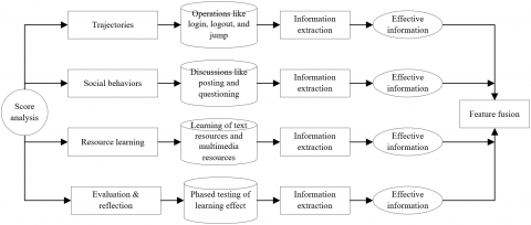
According to the data fusion theory on the big data of education and teaching, the multi-source data of OLP learners were divided into five categories: trajectories, social behaviors, resource learning, evaluation & reflection, and basic information. The features of these types of data were defined, extracted, and fused (Figure 1).
Figure 1. The feature definition, extraction, and fusion of multi-source OLP data
Table 1. The features extracted from OLP learner scores
|
Computational features |
Statistical features |
|
Stay time in school hours |
Number of views of learning resources for major courses |
|
Stay time on holidays |
Number of views of learning resources for other resources |
|
Number of resource learnings on holidays |
Number of assignments |
|
Number of learnings at night |
Test score |
|
Attendance rate of compulsory courses |
Number of discussions |
Note: School hours, a.k.a. regular study hours, refer to 7:30-17:30 on every workday.
The trajectories, the most basic and common data in the OLP, refer to the various operations by learners in the OLP, including login, logout, jump between webpages, and closing webpages.
In terms of social behaviors, every learner can communicate with teachers and other learners in classroom learning on the OLP. The main social behaviors are discussions like real-time posting, questioning, replying, and commenting.
Resource learning dominates the behaviors of OLP learners. The OLP mainly provides two kinds of learning resources: text resources (e.g. PDF and Word), and multimedia resources (e.g. videos, and micro lectures. The learning of text resources involves operations like start, exit, and stay. The learning of multimedia resources involves operations like start, pause, fast forward, loop playback, and stop.
Evaluation & reflection stands for the phased testing of the learning effect on quizzes, assignments, and evaluations. The learning situation of a learner can be reflected comprehensively, if the his/her answering process is preserved on the OLP.
The basic information covers the following personal information of learners: major, student identity (ID), and timetable. Table 1 lists the features extracted from OLP learner scores.
To extract the computational features from the above data, sets A and B were defined as the set of learning resources provided by the OLP, and the set of learning resources for the major, respectively:
$A=\{{{a}_{1}},{{a}_{2}},...,{{a}_{i}},{{a}_{i+1}},...,{{a}{N}}\}$ (1)
$B=\{{{b}_{1}},{{b}_{2}},...,{{b}_{j}},{{b}_{j+1}},...,{{b}_{M}}\}$ (2)
where, ai and bi are the i-th learning resource provided by the OLP and the learning resources for the major of the j-th learner, respectively. In a D-day-long q-th period, the trajectories of the j-th learner can be described by a two-tuple (Pqj, tqj), where Pqj is the stop position of the learning trajectories after the fusion of multi-source learner data, and t is the time that the learner appears in that position. Then, the stop positions of all the trajectories of the j-th learner in the q-th period can be expressed as a set P:
$P=\{{{p}_{1}},{{p}_{2}},...,{{p}_{i}},{{p}_{i+1}},...,{{p}_{K}}\}$ (3)
where, pi is the i-th stop position with a stay time longer than 10min in the trajectories. Next, the OLP learner score features were defined:
(1) Stay time in school hours T1q
In the q-th period of school hours, the positions of learner trajectories that stop at the learning resources of his/her major can be expressed as the following set:
$\begin{align} & P_{maj1}^{qj}=\{{{p}_{i}}\left| for \right.\text{ }each\text{ }{{p}_{i}}\text{ }\in \text{ }P\text{ }\cap \text{ }B\text{ }and\text{ }{{t}^{qj}}\text{ } \in [7:30,17:30]\} \\ \end{align}$ (4)
The stay time at each stop position can be expressed as:
$T_{maj1}^{qj}=\{{{t}_{1}},{{t}_{2}},...,{{t}_{i}},{{t}_{i+1}},...,{{t}_{L}}\}$ (5)
where, t'i is the stay time at the i-th stop position.
The capacity of Pqjmaj1 can be described as:
${{C}_{1}}=\left| P_{maj1}^{qj} \right|$ (6)
Thus, T1q can be defined as:
${{T}_{1q}}=\sum\limits_{i=1}^{L}{{{t}_{i}}}$ (7)
(2) Stay time on holidays T2q
Similar to T1q, in the q-th period of holidays, the positions of learner trajectories that stop at the learning resources of his/her major can be expressed as the following set:
$\begin{align} & P_{maj2}^{qj}=\{{{p}_{i}}\left| for \right. each {{p}_{i}}\in P\cap A and {{t}^{qj}}\text{ } \in holiday\} \\ \end{align}$ (8)
The stay time at each stop position can be expressed as:
$T_{maj2}^{qj}=\{{{{t}'}_{1}},{{{t}'}_{2}},...,{{{t}'}_{i}},{{{t}'}_{i+1}},...,{{{t}'}_{L}}\}$ (9)
where, t'i is the stay time at the i-th stop position.
The capacity of Pqjmaj2 can be described as:
${{C}_{2}}=\left| P_{maj2}^{qj} \right|$ (10)
Thus, T2q can be defined as:
${{T}_{2r}}=\sum\limits_{i=1}^{l}{t_{1}^{'}}$ (11)
(3) Number of resource learnings on holidays N1q
The number of resource learnings on holidays is the capacity of Pqjmaj2:
${{N}_{1q}}={{C}_{2}}$ (12)
(4) Number of learnings at night N2q
Based on the definition of school hours, the period of night learning was limited to 19:30-22:30 at night. The state of night learning NSi was defined as follows: If a learner stops at the learning resources of his/her major in the q-th period and the specified period, then he/she learns at night (NSi=1); otherwise, he/she does not learn at night (NSi=0):
$N{{S}_{i}}=\left\{ \begin{align} & 1,if\text{ }{{t}^{qj}}\in [19:30,22:30]\text{ }and\text{ }{{P}^{qj}}\in A \\ & 0\text{ otherwise} \\ \end{align} \right.$ (13)
The number N2q of learnings at night in a semester can be calculated by:
${{N}_{2r}}=\sum\limits_{i=1}^{D}{N{{S}_{i}}}$ (14)
(5) Attendance rate of compulsory courses ATTL
The attendance in public compulsory courses can basically reflect the overall attendance in all courses. Therefore, the attendance rates of OLP learners in compulsory courses were calculated for different periods in one semester. For the j-th learner, the start and end times of compulsory courses in the q-th period can be calculated by:
$\begin{align} & T_{cou}^{qj}=\{(t_{1}^{b},t_{1}^{e}),(t_{2}^{b},t_{2}^{e}),...,(t_{i}^{b},t_{i}^{e}),(t_{i+1}^{b},t_{i+1}^{e}) ,...,(t_{H}^{b},t_{H}^{e})\} \\ \end{align}$ (15)
${{C}_{3}}=\left| t_{cou}^{qj} \right|$ (16)
where, tbi and tei are the start and end times of the i-th course, respectively. Then, the positions of online courses at each time point in set Tqjcou can be described by the following set:
$W=\{{{w}_{1}},{{w}_{2}},...,{{w}_{i}},{{w}_{i+1}},...,{{w}_{H}}\}$ (17)
For the accuracy of attendance rate, the course duration was expanded 8min before and after the start and end times, creating the range of online time for learners. Then, the attendance rate ATTl of the l-th compulsory course can be defined as:
$AT{{T}_{l}}=\left\{ \begin{align} & 1,if\text{ }{{t}^{qj}}\in [t_{1}^{b}-8,t_{i}^{e}+8]\text{ }and\text{ }{{P}^{qj}}={{w}_{i}} \\ & 0,\text{ otherwise} \\ \end{align} \right.$ (18)
$AT{{T}_{L}}=\left( \sum\limits_{l=1}^{H}{AT{{T}_{l}}} \right)/{{C}_{3}}$ (19)
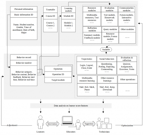
After the computing and extracting the computational and statistical features, the score features of OLP learners can be modelled as Figure 2.
The scores on OLPs are private data of the learners. The acquisition of these data brings certain risks and difficulties. Considering the universality of relevant analysis methods and the predefined features of OLP learner scores, this paper decides to analyze learner scores through EM clustering, which has the advantages of unsupervised learning. The workflow of EM clustering is explained in Figure 3.
The EM clustering is an iterative algorithm based on maximum posterior probability and maximum likelihood estimation. Suppose dataset Z=(X, Y) encompasses observed data X and unobserved data Y, and JPD(X,Y|Ψ) be the joint probability density of these data. Then, finding the maximum of the likelihood function LF (X; Ψ) of X is to make the maximum likelihood estimation of Ψ:
$LF(X;\Psi )=\log JPD(X\left| \Psi \right.)=\int{\log JPD(X,Y\left| \Psi )dY \right.}$ (20)
Figure 2. The model of score features for OLP learners
Figure 3. The workflow of EM clustering
In EM clustering, the EM of LF*(X; Ψ) is iteratively calculated to maximize the log likelihood function of X:
$L{{F}^{*}}(X;\Psi )=\log JPD(X,Y\left| \Psi ) \right.$ (21)
After t iterations, the likelihood estimate of Ψ can be expressed by Ψ(t). During the t+1-th iteration, the likelihood function expectation of Z during the calculation of the posterior probability of each sample belonging to each class can be described as:
$LFE(\Psi \left| \Psi (t) \right.)=PPC\{L{{F}^{*}}(\Psi ;Z)\left| X \right.\left| \Psi (t)\} \right.$ (22)
where, PPC {} is the posterior probability calculation function. During the updating of the probability distribution function of each class through maximum likelihood estimation, LFE (Ψ|Ψ|(t)) is maximized, and Ψ is updated.
The above steps are repeated iteratively to optimize and update model parameters. In this way, the likelihood probability of the training samples and model parameters continues to increase until reaching the extreme point.
After clustering, it is necessary to select suitable features of OLP learner scores. Otherwise, there will be no basis for subsequent data mining. Inspired by the idea of dimensionality reduction, this paper transforms multiple features of OLP learner scores into a few representative features through PCA.
Let Z=(z1,z2,…,zg)T be a g-dimensional random vector obtained by standardizing the original observed data. Then, a matrix of U samples zi=(zi1,zi2,…,zig)T was constructed, and the matrix elements were standardized by:
${{S}_{ij}}=\frac{{{z}_{ij}}-{{{\bar{z}}}_{j}}}{\sqrt{\frac{\sum\limits_{j=1}^{U}{{{({{z}_{ij}}-{{{\bar{z}}}_{j}})}^{2}}}}{U-1}}}$ (23)
${{\bar{z}}_{j}}=\frac{\sum\limits_{i=1}^{U}{{{z}_{ij}}}}{U}$ (24)
The correlation coefficient matrix can be established as:
$R={{[{{r}_{ij}}]}_{g}}=\frac{{{S}^{T}}S}{U-1}={{\left[ \frac{\sum{{{s}_{kj}}\cdot {{s}_{jk}}}}{U-1} \right]}_{g}}$ (25)
Solving the characteristic equation |R-λIg| of formula (25), a total of g characteristic roots can be obtained. The PCA needs to satisfy the following inequality:
${\sum\limits_{j=1}^{d}{{{\lambda }_{j}}}}/{\sum\limits_{j=1}^{g}{{{\lambda }_{j}}}}\;\ge 0.8$ (26)
Then, the d value of principal components with a utilization rate greater than 0.8 was calculated. Solving the equation set Rb=λjb, the unit eigenvector σ0j was obtained. Next, the standardized data features were converted into principal components:
$P{{C}_{ij}}=S_{i}^{T}\sigma _{j}^{0}$ (27)
Taking the variance contribution rate as the weight, the d principal component features were weighted and summed to derive the comprehensive evaluation of OLP learner scores.
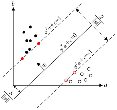
During the analysis and differentiation of OLP learner scores, unsupervised learning can avoid the disclosure of private information like score ranking. However, unsupervised learning cannot accurately distinguish between learners in different score intervals, making the classified management of learners less scientific and effective. Therefore, this paper combines unsupervised EM clustering with supervised SVM (Figure 4) to re-analyze and predict the OLP learner scores.
Figure 4. The principle of the SVM algorithm
Let $f(a)=\varphi^{T} a+c$ be the discriminant function of the $\mathrm{SVM}$ $f(a)=0$ be a two-dimensional (2D) hyperplane that divides all feature samples into two classes, and $\left(a_{1}, b_{1}\right),\left(a_{2}, b_{2}\right), \ldots\left(a_{V},\right.$ by) be the $\mathrm{V}$ feature samples $(b i=+1$ or -1$)$. Then, the classification formula can be defined as:
$\left\{ \begin{matrix} {{\phi }^{T}}a+c\ge 0,{{b}_{i}}=+1 \\ {{\phi }^{T}}a+c<0,{{b}_{i}}=-1 \\\end{matrix} \right.$ (28)
Changing the modulus of the weight vector, the classification rules can be updated as:
$\left\{ \begin{matrix} {{\phi }^{T}}a+c\ge \delta >0\to {{\phi }^{T}}a+c\ge 1,{{b}_{i}}=+1 \\ {{\phi }^{T}}a+c\le -\delta <0\to {{\phi }^{T}}a+c\le -1,{{b}_{i}}=-1 \\\end{matrix} \right.$ (29)
Merging the above formulas:
${{b}_{i}}({{\phi }^{T}}a+c)\ge 1$ (30)
The distance from a to the hyperplane F must be greater than 1:
$\left| g({{a}_{i}}) \right|\ge 1$ (31)
The geometric interval from a sample point to the hyperplane F can be described as:
$\frac{{{b}_{i}}({{\phi }^{T}}a+c)}{\left\| \phi \right\|}$ (32)
where, the numerator $b_{i}\left(\varphi^{T} a+c\right)$ is the interval from the sample point to the hyperplane function. Let γ be the vector perpendicular to the hyperplane F, and υ be the vertical distance between a and F. Following the principle of vector addition, vector a can be rewritten as:
$a=\frac{{{a}_{p}}+\upsilon \phi }{\left\| \phi \right\|}$ (33)
$f(a)={{\phi }^{T}}({{a}_{p}}+\frac{\upsilon \phi }{\left\| \phi \right\|})+c=\upsilon \left\| w \right\|\phi $ (34)
To maximize the interval between the two classes, ||φ|| should be minimized, that is, ||φ||2 should be minimized. However, there exists a constraint |f(a)≥1|, indicating that the sample point closest to the hyperplane represented by the support vector needs to satisfy |f(a)=1|.
According to the concept of data interval, the distance between two sample classes can be defined as 2/||φ||. To minimize ||φ||/2, i.e. maximize the inter-class distance, it is necessary to configure the optimal hyperplane constraint, that is, the optimization function of SVM:
$\underset{\phi }{\mathop{\text{min}}}\,\frac{1}{\left\| \phi \right\|_{2}^{{}}}\text{ }s.t.\text{ }{{b}_{i}}({{\phi }^{T}}a+c)\ge 1$ (35)
After finding the support vector and maximizing the interval, φ and c can be determined. Then, the optimization function is equivalent to:
$\arg \underset{\phi c}{\mathop{\max }}\,\left\{ \underset{\phi }{\mathop{\min }}\,({{\phi }^{T}}{{a}_{i}}+c))\frac{1}{\left\| \phi \right\|} \right\}$ (36)
Since linear classification cannot differentiate all actual samples, the few misclassified samples were separated with a slack variable:
$\min \frac{1}{2}{{\left\| \phi \right\|}^{2}}+\eta \sum\limits_{i=1}^{n}{{{\mu }_{i}}}\text{ }s.t.\text{ }{{b}_{i}}({{\phi }^{T}}a+c)\ge 1-{{\mu }_{i}},{{\mu }_{i}}\ge 0$ (37)
where, μi is the slack variable; η is a constant, representing the penalty function. If misclassified, sample a can be discarded if the η value is sufficiently small. The smaller the η value, the wider the hyperplane, and the more the misclassified sample points. This problem can be solved by introducing the Lagrangian factor to hyperplane optimization. The Lagrangian optimization function can be constructed as:
$\begin{align} & \max L(\phi ,c,\alpha )=\frac{1}{2}({{\phi }^{T}}\phi )-\sum\limits_{i=1}^{V}{{{\alpha }_{i}}}\left[ {{b}_{i}}({{\phi }^{T}}{{a}_{i}}+c)-1 \right] \\ & s.t.\text{ }0\le {{\alpha }_{i}}\le \eta \\ \end{align}$ (38)
Finding the partial derivatives:
$\left\{ \begin{matrix} \frac{\partial L(\phi ,c,\alpha )}{\partial \phi }=0\text{ }\Leftrightarrow \text{ }\phi -\sum\limits_{i=1}^{V}{{{\alpha }_{i}}}{{b}_{i}}{{a}_{i}}=0 \\ \frac{\partial L(\phi ,c,\alpha )}{\partial c}=0\text{ }\Leftrightarrow \text{ }\sum\limits_{i=1}^{V}{{{\alpha }_{i}}}{{b}_{i}}=0 \\\end{matrix} \right.$ (39)
Combining formulas (38) and (39):
$L(\phi ,c,\alpha )=\sum\limits_{i=1}^{V}{{{\alpha }_{i}}}-\frac{1}{2}\sum\limits_{i=1}^{V}{\sum\limits_{j=1}^{V}{{{\alpha }_{i}}{{\alpha }_{j}}{{b}_{i}}{{b}_{j}}a_{i}^{T}{{a}_{j}}}}$ (40)
The optimal solution αi* can be obtained by taking the maximum of the above formula. The optimal constraint can be described as:
$\text{ }{{\phi }^{*}}=\sum\limits_{i}^{{{V}_{S}}}{\alpha _{i}^{*}}{{b}_{i}}{{a}_{i}}$ (41)
where, VS is the number of support vectors. The optimal bias can be obtained by:
${{c}^{*}}={{b}_{i}}-{{\phi }^{*T}}{{a}_{i}}$ (42)
Solving the Lagrangian factor αi, the optimal hyperplane can be easily obtained.
The massive data on OLP learner behaviors were collected and processed through the flow in Figure 5, and the preprocessed features were stored in a non-relational database. The learner behavior data involve attributes like StudentID, SessionID, Verb, Object, and Context, which help to judge whether a learner enters a session or exit the system.
Figure 5. The collection and preprocessing of learner behavior data
The originally extracted data contain lots of redundant information. The high-quality features need to be selected from the original data, such that the model will not face problems induced by the curse of dimensionality: poor generalization, high complexity, and long training. Here, the correlation coefficients of score features in each category are calculated by the correlation coefficient method. The calculated results are recorded in Table 2.
If the Pearson correlation coefficient falls in 0.5-1.0, the features are strongly correlated; if the coefficient falls in 0.3-0.5, the features are moderately correlated; if the coefficient falls in 0.1-0.3, the features are slightly correlated; if the coefficient falls in 0-0.1, the features are basically uncorrelated. This paper chooses the features with Pearson correlation coefficient greater than 0.3 for clustering analysis.
Table 2. The salient features of OLP learner scores and their Pearson correlation coefficients
|
Computational features |
Correlation coefficient |
Statistical features |
Correlation coefficient |
|
Stay time in school hours |
0.431 |
Total number of visits to multimedia resources |
0.321 |
|
Stay time on holidays |
0.411 |
Total number of visits to text resources |
0.311 |
|
Number of resource learnings on holidays |
0.382 |
Score of unit quiz |
0.316 |
|
Number of learnings at night |
0.341 |
Number and quality of assignments |
0.357 |
|
Attendance rate of compulsory courses |
0.391 |
Forum activity |
0.382 |
|
|
|
Number of interactions with teachers |
0.326 |
|
|
|
Number of notes and feedbacks |
0.346 |
|
|
|
Self-evaluation |
0.391 |
|
|
|
Student-student mutual evaluation |
0.325 |
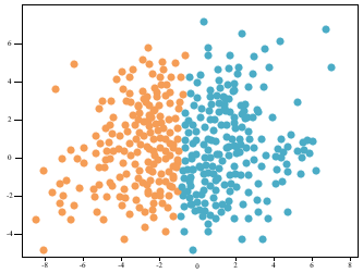
(a) Two classes
(b) Three classes
Figure 6. The visualized results of EM clustering of selected features
From the multi-source data of OLP learners throughout the 20-week semester, the features closely correlated with learner scores were extracted, and grouped by EM clustering into two classes (I and II) or three classes (I, II, and III). To give a visual display of the clustering results, the features to be clustered were subject to PCA and dimensionality reduction. The visualized results of EM clustering are displayed in Figure 6.
Following the idea of equal division, the results of three-class EM clustering before and after feature selection were divided into three levels, namely, 1-200, 200-400, and 400-600, and the clustering accuracy in each level was calculated in turn. Table 3 compares the accuracies of EM clustering before and after feature selection.
From Figure 6 and Table 3, the EM clustering achieved a good effect on the OLP learner scores. The accuracy before feature selection was higher than that after feature selection. The three-class clustering was more accurate than two-class clustering, with accuracy falling between 82.76% and 86.74%. Therefore, our clustering analysis method excels in distinguishing fine-grained features of learner scores.
Next, three SVM classifiers were designed by integrating multiple binary classifiers through one-against-one. Their performance was cross validated, and evaluated. Then, the SVM classifiers were adopted to predict the multiple classes of learner scores, based on the feature subset of the multi-source data on OLP learner scores and the features closely correlated with learner scores. Table 4 compares the classification results of the three SVM classifiers.
It can be seen that the three-class SVM classifier achieved an accuracy of 82-91%, slightly higher than that of two-class SVM classifier. This classifier effectively distinguished between the scores of learners in different levels, suggesting that it is suitable for analyzing and managing OLP learner scores.
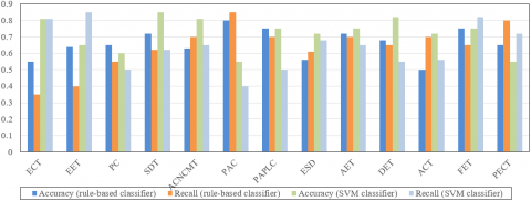
Furthermore, the scores of electrical automation majors on 13 professional courses were clustered by the proposed SVM classifier and the rule-based classifier. As shown in Figure 7, the proposed SVM classifier outshined the rule-based classifier in accuracy and recall, despite a slight lag in efficiency. The results demonstrate the accuracy and effectiveness of our method in the classification of OLP learners and their score features.
Table 3. The EM clustering accuracies before and after feature selection
|
Levels |
I |
Ⅱ |
Ⅲ |
|||
|
Before feature selection |
After feature selection |
Before feature selection |
After feature selection |
Before feature selection |
After feature selection |
|
|
1-200 |
59 |
61 |
20 |
21 |
74 (positive samples) |
76 (positive samples) |
|
200-400 |
84 (positive samples) |
96 (positive samples) |
62 |
59 |
52 |
58 |
|
400-600 |
41 |
39 |
80 (positive samples) |
92 (positive samples) |
24 |
26 |
|
Accuracy |
82.76% |
82.91% |
84.82% |
86.74% |
82.74% |
85.74% |
Table 4. The classification results of the 3 SVM classifiers before and after feature extraction
|
Type |
Accuracy |
Recall |
F1-score |
Support |
||||
|
Before feature selection |
After feature selection |
Before feature selection |
After feature selection |
Before feature selection |
After feature selection |
Before feature selection |
After feature selection |
|
|
I |
0.87 |
0.89 |
0.19 |
0.21 |
0.24 |
0.29 |
16 |
21 |
|
Ⅱ |
0.82 |
0.85 |
0.92 |
0.94 |
0.78 |
0.82 |
58 |
59 |
|
Ⅲ |
0.87 |
0.91 |
0.16 |
0.22 |
0.34 |
0.46 |
22 |
22 |
Figure 7. The classification results on professional course scores of rule-based classifier and SVM classifier
Note: ECT is Electrical Control Technology, EET is Electrical and Electronic Technology, PC is Programmable Controller, SDT is Sensing and Detection Technology, ACNCMT is Application of Computer Numerically Controlled (CNC) Machine Tools, PAC is Principle of Automatic Control, PAPLC is Principle and Application of Programmable Logic Controller (PLC), ESD is Electronic System Design, AET is Analog Electronic Technology, DET is Digital Electronic Technology, ATC is Application of Computer Technology, FET is Fundamentals for Electrical Towage, PECT is Power Electronic Conversion Technology.
Based on data mining, this paper develops a course score analysis model for OLS learners. Firstly, the score features of OLS learners were categorized, and the calculation method for computational features was detailed. Then, EM clustering was adopted to cluster the score features of the learners, owing to its advantage of unsupervised learning. The salient features were obtained through PCA. Experimental results demonstrate that our clustering analysis method excels in distinguishing fine-grained features of learner scores. Finally, the authors designed an SVM classifier, a supervised learning tool, and combined it with EM clustering to accurately categorize the score features of OLS learners. The proposed method was compared with the rule-based classifier. The comparison shows that our method achieved the better accuracy and recall, an evidence to its feasibility and accuracy.
[1] Mahmud, M., Nor, N.M., Jauhari, N.E., Nordin, N.I., Rahman, N.A. (2020). Student engagement and attitude in mathematics achievement using single valued neutrosophic set. Journal of Physics: Conference Series, 1496(1): 012017. https://doi.org/10.1088/1742-6596/1496/1/012017
[2] Faber, J.M., Luyten, H., Visscher, A.J. (2017). The effects of a digital formative assessment tool on mathematics achievement and student motivation: Results of a randomized experiment. Computers & Education, 106: 83-96. https://doi.org/10.1016/j.compedu.2016.12.001
[3] Yildirim, I. (2017). The effects of gamification-based teaching practices on student achievement and students' attitudes toward lessons. The Internet and Higher Education, 33: 86-92. https://doi.org/10.1016/j.iheduc.2017.02.002
[4] Masson, A.L., Klop, T., Osseweijer, P. (2016). An analysis of the impact of student–scientist interaction in a technology design activity, using the expectancy-value model of achievement related choice. International Journal of Technology and Design Education, 26(1): 81-104. https://doi.org/10.1007/s10798-014-9296-6
[5] Giridharan, P.K., Raju, R. (2016). The impact of experiential learning methodology on student achievement in mechanical automotive engineering education. International Journal of Engineering Education, 32(6): 2531-2542.
[6] Asarta, C.J., Schmidt, J.R. (2017). Comparing student performance in blended and traditional courses: Does prior academic achievement matter? The Internet and Higher Education, 32: 29-38. https://doi.org/10.1016/j.iheduc.2016.08.002
[7] Popyack, J.L. (2016). UPSILON PI EPSILON UPE 2016 national meeting, and celebrating outstanding student achievement. ACM Inroads, 7(2): 28-30. https://doi.org/10.1145/2926716
[8] Mabed, M., Köhler, T. (2016). Aligning performance assessments with standards: A practical framework for improving student achievement in vocational education. Knowledge, Information and Creativity Support Systems, 416: 575-585. https://doi.org/10.1007/978-3-319-27478-2_45
[9] Rahman, K., Qodriyah, K., Bali, M.M.E.I., Baharun, H., Muali, C. (2020). Effectiveness of android-based mathematics learning media application on student learning achievement. Journal of Physics: Conference Series, 1594(1): 012047. https://doi.org/10.1088/1742-6596/1594/1/012047
[10] Apriesnig, J.L., Manning, D.T., Suter, J.F., Magzamen, S., Cross, J.E. (2020). Academic stars and energy stars, an assessment of student academic achievement and school building energy efficiency. Energy Policy, 147: 111859. https://doi.org/10.1016/j.enpol.2020.111859
[11] Wibowo, A.N., Wibowo, Y.E. (2020). Implementing student teams-achievement division to improve student’s activeness and achievements on technical drawing courses. Journal of Physics: Conference Serie, 1446(1): 012033. https://doi.org/10.1088/1742-6596/1446/1/012033
[12] Apuanor, S., Yuniarsih, R.O. (2020). The influence of library and internet utilization of student achievement index. Journal of Physics: Conference Series, 1477(4): 042026. https://doi.org/10.1088/1742-6596/1477/4/042026
[13] Rustana, C.E., Andriana, W., Serevina, V., Junia, D. (2020). Analysis of student’s learning achievement using PhET interactive simulation and laboratory kit of gas kinetic theory. Journal of Physics: Conference Series, 1567(2): 022011. https://doi.org/10.1088/1742-6596/1567/2/022011
[14] Wasil, M., Sudianto, A. (2020). Application of the decision tree method to predict student achievement viewed from final semester values. Journal of Physics: Conference Series, 1539(1): 012027. https://doi.org/10.1088/1742-6596/1539/1/012027
[15] Sebillo, M., Vitiello, G., Di Gregorio, M. (2020). Maps4Learning: Enacting geo-education to enhance student achievement. IEEE Access, 8: 87633-87646. https://doi.org/10.1109/ACCESS.2020.2993507
[16] Sudipa, I.G.I., Wijaya, I.N.S.W., Radhitya, M.L., Mahawan, I.M.A., Arsana, I.N.A. (2020). An android-based application to predict student with extraordinary academic achievement. Journal of Physics: Conference Series, 1469(1): 012043. https://doi.org/10.1088/1742-6596/1469/1/012043
[17] Lerche, T., Kiel, E. (2018). Predicting student achievement in learning management systems by log data analysis. Computers in Human Behavior, 89: 367-372. https://doi.org/10.1016/j.chb.2018.06.015
[18] Setyowati, C.S.P., Louise, I.S.Y. (2018). Implementation of reflective pedagogical paradigm approach on the rate of reaction to student achievement. Journal of Physics: Conference Series, 1097(1): 012057. https://doi.org/10.1088/1742-6596/1097/1/012057
[19] Dahri, S., Yusof, Y., Chinedu, C. (2018). TVET lecturer empathy and student achievement. Journal of Physics: Conference Series, 1049(1): 012056. https://doi.org/10.1088/1742-6596/1049/1/012056
[20] Syahidi, A.A., Asyikin, A.N. (2018). Applying student team achievement divisions (STAD) model on material of basic programme branch control structure to increase activity and student result. IOP Conference Series: Materials Science and Engineering, 336(1): 012027. https://doi.org/10.1088/1757-899X/336/1/012027
[21] Hamdi, S., Kartowagiran, B. (2020). Learning achievement of Elementary School student of mathematics using the Testlet model instrument: A comparison between the 2006 Curriculum and the 2013 Curriculum. Journal of Physics: Conference Series, 1581(1): 012055. https://doi.org/10.1088/1742-6596/1581/1/012055
[22] Arami, M., Wiyarsi, A. (2020). The student metacognitive skills and achievement in chemistry learning: correlation study. Journal of Physics: Conference Series, 1567(4): 042005. https://doi.org/10.1088/1742-6596/1567/4/042005
[23] Wibawa, S.C. (2018). The impact of fashion competence and achievement motivation toward college student’s working readiness on “Cipta Karya” subject. In Materials Science and Engineering Conference Series, 296(1): 012017. https://doi.org/10.1088/1757-899X/296/1/012017
[24] Gkontzis, A.F., Kotsiantis, S., Tsoni, R., Verykios, V.S. (2018). An effective LA approach to predict student achievement. Proceedings of the 22nd Pan-Hellenic Conference on Informatics, New York, US, pp. 76-81. https://doi.org/10.1145/3291533.3291551
[25] Northey, G., Govind, R., Bucic, T., Chylinski, M., Dolan, R., Van Esch, P. (2018). The effect of “here and now” learning on student engagement and academic achievement. British Journal of Educational Technology, 49(2): 321-333. https://doi.org/10.1111/bjet.12589