Zaihua Yang
© 2020 IIETA. This article is published by IIETA and is licensed under the CC BY 4.0 license (http://creativecommons.org/licenses/by/4.0/).
OPEN ACCESS
With the continuous urbanization in China, the number of private cars has grown rapidly in urban areas, leading to increasingly prominent road congestions. Urban road networks are wide but sparse, which can easily cause congestion. To tackle with this problem, the State Council proposed the idea of “open residential community” in 2016, which is to connect the roads within the residential community with external roads to densify the road networks and increase the area of branch roads, so as to mitigate urban road traffic pressure. In order to study the impacts of open residential communities on the traffic capacity of surrounding roads, this paper first establishes an evaluation indicator system for road traffic using a number of factors such as traffic density, traffic delay time, number of intersection conflicts, road congestion rate and road accessibility based on the analytic hierarchy process (AHP) theory, and also builds a fuzzy comprehensive evaluation model. Then, with the above evaluation indicator system and model, this paper employs the VISSIM traffic simulation technology to simulate the residential community for testing. Finally, it uses the grey relational algorithm to compare and analyze the test data, and obtains the following conclusions: for residential communities with a large area and large traffic volume and those with a small area and large traffic volume, the surrounding road traffic is significantly reduced, and the traffic pressure is greatly alleviated; the effect comes second for those with a large area and small traffic volume; and for those with a small area and small traffic volume, surrounding traffic sees no improvement.
open residential community, AHP, fuzzy comprehensive evaluation, VISSIM traffic simulation
Traffic congestion in China has been a difficult problem nowadays. One of the important causes for this situation is the road layout model where roads are wide and networks are sparse. In road construction, urban trunk roads take up the vast majority of road areas, while branch roads are far from enough, which is the exact opposite of the “small blocks and dense road networks” model advocated in Western countries today. Large-size residential communities which passing vehicles have no access to is one of the important reasons resulting in the reasonable road structure and network density. With the emergence of various new theories of urban development planning in the United States in the 1980s, the new idea and theories of “open dwellings” began to spread around the world [1,2]. In fact, a number of theories on urban planning and urban spatial structure already took shape in the U.S. and Europe as early as in the 1920s, while there has hardly been any innovative theoretical system in China.
It requires systematic evaluation to figure out whether the road traffic conditions around a residential community will be truly improved after the community is opened. Analytic hierarchy process and fuzzy comprehensive evaluation method are common methods used to evaluate complex systems for decision-making. In recent years, scholars and forerunners at home and abroad have done some exploration and research on both methods. Guegan et al. [1] applied AHP in the ranking of traffic smoothing projects as an alternative to the existing scoring system. The ranking produced by the AHP is different from those by other methods. When certain factors cannot be quantified, the AHP will show its advantages. Gong and Li [2] applied Delphi and AHP in the analysis of various factors affecting road transport safety and proposed an indicator system suited to road transport enterprises in China. The comprehensive evaluation results can be applied in actual situations to reflect road transportation safety. Aiming at how to contact the nearest rescue organization as soon as possible so as to reduce casualties and property losses in the event of a traffic accident in an urban area, Chang et al. [3] developed an intelligent GIS rescue system using AHP to indicate the fastest route to the accident scene. Wang and Liu [4] used the AHP and the fuzzy comprehensive evaluation method to optimize the design schemes of energy-saving houses. They established the hierarchical structure of the energy-saving house design schemes through analysis, calculated the universally applicable hierarchical total ranking weight vector, and finally provided references for the optimization of energy-saving house design schemes. Wang and Zhang [5] used the AHP - entropy weight method and the fuzzy comprehensive evaluation method to evaluate the suitability of construction land. The three-scale method used in weight determination solves the consistency test problem of the traditional nine-scale method to some extent, and it is easier for scoring and more operable. Yu et al. [6] established an evaluation indicator system for traffic congestion at urban road intersections by applying the analytic hierarchy process, and evaluated traffic conditions at intersections and made decisions using the prioritization technique similar to the ideal solution TOPSIS. Nosal and Soleck [7] used the Multi-Criteria Decision Analysis (MCDA) method to evaluate various variants of the integrated system of urban public transport (ISUPT). In the evaluation, they used one of the MCDA methods - AHP, showing a different way of integration. Żak and Kruszyński [8] carried out multi-level, multi-index evaluation on 18 urban transport projects, and applied AHP, ELECTRE III/IV and their combinations (AHP / ELECTRE III/IV) at each level of the hierarchical decision-making problem to construct and solve different multi-criteria ranking sub-problems. Barić et al. [9] used a multi-index analytic hierarchy process to evaluate the design of road segments in an urban environment. By weighting different evaluation indices and sub-indices, the evaluation provided reliable results and proved to be robust for sensitive analysis. Li et al. [10] proposed an AHP-based method to determine the weights of the influencing factors to decision-making, took into account their relative importance, and comprehensively ranked each road segment. Taking the highway network maintenance priority as an example, they illustrated the feasibility of this method. Mei et al. [11] pointed out the infeasibility of the previous weight determination and evaluation result expression method in fuzzy comprehensive evaluation of water quality, and proposed new methods for weight determination and evaluation result expression, so that fuzzy comprehensive evaluation has more realistic meaning. They also verified these methods with examples. Regarding the problem that it is difficult to accurately identify the source of gushing water with just one single factor, Yu et al. [12] established a two-level fuzzy comprehensive evaluation mathematical model based on underground aquifer water chemical analysis and gushing water data, which can accurately identify underground gushing water sources, showing that it has some practical value. Wang and Huo [13] applied the fuzzy comprehensive evaluation method in the safety evaluation of the coal industry based on the fuzzy mathematics theory, established a coal safety evaluation system according to the current status of coal safety, adopted AHP to determine relative weights and calculated the safety grade characteristic quantity. Shao et al. [14] used the analytic hierarchy process to establish a scheme selection model for the construction of a sewage treatment plant in Zhongshan City and sought to optimize the decision. Through optimization calculation using the AHP method and the fuzzy comprehensive evaluation based on the actual situation of the water treatment system, they finally obtained the optimal scheme. Yang et al. [15] introduced the analytic hierarchy process to the comprehensive evaluation on the simulation credibility of the underwater vehicle system, and determined the weight of each factor in the system simulation credibility evaluation indicator system.
This paper first establishes an evaluation indicator system from three aspects - road capacity, road safety and road vulnerability. Through multiple screenings, this paper decides to select 5 indicators, namely traffic density, traffic delay time, number of intersection conflicts, road congestion rate and road accessibility to reflect the surrounding road traffic conditions before and after a residential community is opened. Then, based on these indicators, this paper establishes an analytic hierarchy structure model, calculates the weights of these indicators, and passes the consistency check to make sure the reliability of the indicator system. After that, based on the analytic hierarchy model, it establishes a fuzzy comprehensive evaluation model and performs quantitative evaluation on road traffic. At last, based on the above evaluation indicator system and model and by applying the VISSIM traffic simulation technique, this paper performs a simulation test on a residential community and compares and analyze the test results through the grey relational algorithm.
This paper first establishes an evaluation indicator system from three aspects - road capacity, road safety and road vulnerability [16, 17]. After multiple screenings, this paper decides to use five indicators, namely traffic density, traffic delay time, number of intersection conflicts, road congestion rate and road accessibility to reflect the surrounding road traffic conditions before and after the opening of a residential community.
2.1 Description of evaluation indicators
2.1.1 Traffic density
Traffic density refers to the number of vehicles distributed on a unit length of a lane at a certain instant of time, which reflects the concentration degree of vehicle distribution. The calculation formula is as follows:
$\text{K}=\text{N/L (pcu/km) }$ (1)
where, K is the traffic density; N is the number of vehicles on a single-lane road segment (pcu); L is the length of the road segment.
2.1.2 Traffic delay time
The traffic delay time at intersections is one of the important indicators to measure the efficiency of traffic operations. The opening of a residential community may affect the traffic delay time at intersections [18]. Through comparison of the delay time before and after community opening, the impact on road traffic capacity can be obtained.
The calculation formula is as follows:
$\text{W}=\frac{(\rho +\frac{{{\rho }^{2}}+q_{0}^{2}\frac{1}{{{q}^{2}}}}{2(1-\rho )})}{q}$ (2)
where, W is the traffic delay time at the intersection; ρ is the utilization rate (service intensity) of the entrance, which is the ratio of the average number of vehicles arriving at the intersection to the average number of vehicles that can be serviced at the same time, that is, the probability of any vehicle waiting on the stop line at the intersection; q is the average traffic flow at the intersection; and q0 is the specific traffic flow at a certain intersection.
2.1.3 Number of intersection conflicts
The number of intersection conflicts (this paper only studies the situations at intersections with no traffic light) can be used as a safety evaluation indicator [19]. The theoretical formula to estimate the number of conflicts per hour at a road intersection is as follows:
$\text{N}=3600{{H}_{0}}({{\lambda }_{1}}{{e}^{-{{\lambda }_{1}}{{H}_{0}}}})({{\lambda }_{2}}{{e}^{-{{\lambda }_{2}}{{H}_{0}}}})$ (3)
where, N is the number of intersection conflicts (theoretical estimate); and $\lambda_{1}$ and $\lambda_{2}$ are the traffic flow on the trunk road and the branch road (residential community road), respectively; and H0 is the threshold of the time interval between the arrivals of vehicles from the residential community road and the trunk road at the statistical cross section.
2.1.4 Road congestion rate
Road congestion rate is the ratio of the actual traffic volume on a road segment to the evaluation benchmark for 24 hours a day or 12 hours during the daytime [20].
The calculation formula is as follows:
$\text{D}C=\frac{\varpi *\text{Q}}{C}$ (4)
where, $D C$ is the congestion rate; $\varpi$ is the weight coefficient, and $\varpi=1-\alpha / 100+\alpha * \beta / 100 ; \alpha$ is the mixing rate of oversize vehicles; Q is the total traffic volume during the 12-hour daytime; and C is the evaluations benchmark for 12-hour traffic volume.
2.1.5 Road accessibility
Road accessibility refers to the relative difficulty of moving from any point to another point in the road network, and factors related to this indicator include distance, time, cost and so on. Road accessibility in fact reflects the road resistance to a certain horizontal movement process [21]. The overall accessibility of an urban road is expressed as weighted accessibility [22]. It can be calculated as the weighted average of the accessibility of each OD point pair with the traffic load as the weight, that is,
$\gamma =\frac{1}{\sum\limits_{\text{A},B\in l}{{{U}_{AB}}}}\sum\limits_{A,B\in l}{{{U}_{AB}}{{\gamma }_{AB}}}$ (5)
where, $U_{A B}$ is the traffic volume of $A \rightarrow B ; \gamma_{A B}$ is the accessibility of $A \rightarrow B$. With the residential community accessibility as an example, the weighted accessibility indicator can be calculated as:
$\gamma =\frac{1}{\sum\limits_{\text{i}=1}^{I}{\sum\limits_{j=1}^{J}{{{U}_{ij}}}}}\sum\limits_{i=1}^{I}{\sum\limits_{j=1}^{J}{{{U}_{ij}}{{\gamma }_{ij}}}}$ (6)
For ease of expression and calculation, it can be defined that when i=j, $U_{i j}=0, \gamma_{i j}=1$.
2.2 AHP modelling
2.2.1 Establishment of the hierarchy structure
The Analytic Hierarchy Process (AHP) is to decompose the decision problem into different hierarchical levels in the order of overall objectives, sub-objectives at each layer, evaluation criteria and specific schemes, then calculate the priority value of each element on a layer to a certain element on the immediate upper layer by solving the feature vector of the judgment matrix, and at last recursively obtain the final weight of each scheme to the overall objective by the weighted sum method [23]. The one with the largest final weight is the optimal solution.
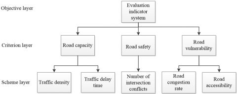
To apply the AHP in the comprehensive evaluation of the impacts of an open residential community on road traffic, a hierarchical analysis model must be established first. Through analysis, it can be known that the indicators affecting road traffic are logically related in a way that sub-class indicators reflect a main class indicator while main class indicators reflect the road traffic capacity. This logical relationship is hierarchical, decomposing elements related to decision-making into objective, criteria and schemes, as shown in Figure 1.
Figure 1. Hierarchy structure
2.2.2 Weight analysis of evaluation indicators based on AHP
The weight of each influencing factor in the criterion layer is determined, forming a pairwise comparison matrix as shown below:
$\text{M}=\left( \begin{matrix} 1 & 3/4 & 4/3 \\ 4/3 & 1 & 3/2 \\ 3/4 & 2/3 & 1 \\\end{matrix} \right)$.
Through calculation with the software MATLAB, the feature vector corresponding to the maximum feature root is:
$\beta=(0.3280 .4130 .260)$.
Consistency check is carried out to determine whether the result is feasible. Through calculation, there is:
$CI=\frac{\lambda \max -n}{n-1}=0$.
The values of the random consistency index RI are shown in Table 1.
Table 1. Values of the consistency index RI
|
n |
1 |
2 |
3 |
4 |
5 |
6 |
7 |
8 |
|
RI |
0 |
0 |
0 |
0.9 |
1.12 |
1.24 |
1.32 |
1.41 |
It shows that the results are feasible. The weights of the influencing factors in the criterion layer are shown in Table 2.
Table 2. Weights of the influencing factors in the criterion layer
|
Indicator |
Weight |
Consistency check |
|
Traffic capacity A |
$\varpi 1$=0.328 |
$\Sigma \varpi_{i}=1 \quad \lambda \max =3$ CI=0 CR=0<0.1 |
|
Safety B |
$\varpi 2$=0.413 |
|
|
Vulnerability C |
$\varpi 3=0.260 |
The weight of each influencing factor in the scheme layer is shown in Table 3.
Table 3. Weight of each influencing factor in the scheme layer
|
Indicator |
Weight |
|
Traffic density |
ω1=0.159 |
|
Traffic delay time |
ω2=0.123 |
|
Traffic saturation |
ω3=0.115 |
|
Number of intersection conflicts |
ω4=0.127 |
|
Road congestion rate |
ω5=0.471 |
2.3 Establishment of the fuzzy comprehensive evaluation model
2.3.1 Overview of the fuzzy comprehensive evaluation model
The fuzzy comprehensive evaluation method is a comprehensive evaluation method based on fuzzy mathematics. It converts qualitative evaluation to quantitative evaluation according to the membership theory of fuzzy mathematics; in other words, it uses fuzzy mathematics to make an overall evaluation of the things or objects restricted by multiple factors. With clear results and strong systematicness, this method can solve problems that are fuzzy and difficult to quantify, and thus is suitable for solving various uncertainty problems. The concept of fuzzy set theory was proposed in 1965 by Professor Chad, the American automatic control expert, to express the uncertainty of things [24].
2.3.2 Basic steps of the fuzzy comprehensive evaluation model
(1) Determine the factor set
Road traffic needs to be comprehensively evaluated from multiple aspects. This paper directly uses the evaluation indicator system previously established as the factor set, which is denoted as:
U={u1, u2, ..., un},
where, ui (i=1, 2, ..., n) represents each influencing factor.
(2) Determine the remark set
Due to the different evaluation results of the indicators, there will be different ratings. For example, for work performance, the ratings include “excellent”, “good”, “medium”, “poor” and “very poor”. The set consisting of different evaluation results is called a remark set, denoted as:
V={v1, v2, ..., vm},
where, vi (i=1, 2, ..., m) represents each rating.
(3) Determine the weight of each factor
In general, different factors in the factor set have different contributions in the comprehensive evaluation. The comprehensive evaluation results are not only related to the evaluation result of each factor, but also dependent to a large extent on how these factors contribute to the comprehensive evaluation. This indicates that the weight distribution of all these factors has to be determined. It is a fuzzy vector on U, denoted as:
A={a1, a2, …, an},
where, ai represents the weight of the i-th factor, which satisfies $\sum_{i=1}^{n} a_{i}=1$. There are many methods for determining the weights, such as the Delphi method, the weighted average method, and the crowd evaluation method etc.
(4) Determine the fuzzy comprehensive judgment matrix
For the indicator ui, each remark is a fuzzy subset on V. The evaluation of the indicator ui is denoted as:
Ri={Ri1, Ri2, ..., Rim},
The fuzzy comprehensive judgment matrix of each indicator is:
$R=\left[ \begin{matrix} {{r}_{11}} & {{r}_{12}} & ... & {{r}_{1m}} \\ {{r}_{21}} & {{r}_{22}} & ... & {{r}_{2m}} \\ ... & ... & ... & ... \\ {{r}_{n1}} & {{r}_{n2}} & ... & {{r}_{nm}} \\\end{matrix} \right]$.
It is a fuzzy relation matrix from U to V.
(5) Perform comprehensive evaluation
If there is a fuzzy relationship from U to V, which is R=(Rij)n×m, then a fuzzy transformation [25] $T_{R}: F(U) \rightarrow F(V)$ can be obtained using R, and from this transformation, the comprehensive evaluation result can be obtained, which is B=A•R.
The comprehensive evaluation can be regarded as a fuzzy vector on V, denoted as B={b1, b2, ..., bm}.
2.3.3 Application of the fuzzy comprehensive evaluation model in this study
(1) Set the factor set as:
U={traffic density u1, traffic delay time u2, number of intersection conflicts u3, road congestion rate u4, road accessibility u5}.
(2) Set the remark set as:
V={good v1, relatively good v2, average v3, relatively poor v4, poor v5}.
(3) Determine the weight of each factor
Based on the weight of each indicator obtained, list the weight vector A={0.159, 0.123, 0.115, 0.127, 0.471}.
(4) Determine the fuzzy comprehensive evaluation matrix, and rate each ui.
For example, u1 is determined based on the score given by the expert panel. Suppose the scores are as follows:
R1=[0.1, 0.2, 0.2, 0.3, 0.2].
The above expression indicates that 10% of the experts participating in the scoring think that the traffic density is good, 50% think that the traffic density is relatively good, 40% think that the traffic density is average, and 0 expert think that the traffic density is relatively poor or poor. The other factors are also evaluated in the same way.
u2, u3, u4 and u5 are also scored by the expert panel:
R2=[0.2, 0.3, 0.5, 0, 0], R3=[0.2, 0.2, 0.4, 0.1, 0.1], R4=[0.1, 0.1, 0.5, 0.3, 0] and R5=[0.2, 0.2, 0.2, 0.2, 0.2].
Let Ri be line i to form the evaluation matrix:
$R=\left[ \begin{matrix} 0.1 & 0.2 & 0.2 & 0.3 & 0.2 \\ 0.2 & 0.3 & 0.5 & 0 & 0 \\ 0.2 & 0.2 & 0.4 & 0.1 & 0.1 \\ 0.1 & 0.1 & 0.5 & 0.3 & 0 \\ 0.2 & 0.2 & 0.2 & 0.2 & 0.2 \\\end{matrix} \right]$.
It is a fuzzy relation matrix from the factor set U to the remark set V.
(5) Fuzzy comprehensive evaluation
Perform compositional operation of the matrix.
B=A•R=[0.159, 0.123, 0.115, 0.127, 0.471]$\left[ \begin{matrix} 0.1 & 0.2 & 0.2 & 0.3 & 0.2 \\ 0.2 & 0.3 & 0.5 & 0 & 0 \\ 0.2 & 0.2 & 0.4 & 0.1 & 0.1 \\ 0.1 & 0.1 & 0.5 & 0.3 & 0 \\ 0.2 & 0.2 & 0.2 & 0.2 & 0.2 \\\end{matrix} \right]$=[0.1704, 0.1986, 0.2970, 0.1915, 0.1373]
According to Table 4, the remark with the greatest value is taken as the comprehensive evaluation result, which is “average”.
Table 4. Evaluation results and ratings
|
Poor |
Relatively poor |
Average |
Relative good |
Good |
|
<0.1 |
[0.1, 0.2) |
[0.2, 0.35) |
[0.35, 0.5) |
≥0.5 |
3.1 Definitions of open residential community types
In most of the research on open residential communities, the internal road structure of the residential community was used as the sole criterion for the classification of residential communities. This paper categorizes residential communities according to the different effects on road traffic. The internal road structure of the residential community is only one of the factors affecting traffic, and not the main factor. The area of the residential community and the traffic volume around the residential community should be treated as the main criteria for the classification of residential communities.
The block-type residential community is the most common form adopted in current residential area planning. This study further divides the block-type residential communities. With area and surrounding traffic volume as the criteria, residential communities are classified into 4 types, namely large area and large traffic volume, large area and small traffic volume, small area and large traffic volume, and small area and small traffic volume (referred to as Type A, Type B, Type C and Type D residential communities respectively in this paper). Definitions of these types of residential communities are listed in Table 5.
Table 5. Definitions of different types of residential communities
|
Type A residential community |
Area of 25-35 ha. (375-525 mu) and high traffic volume |
|
Type B residential community |
Area of 25-35 ha. (375-525 mu) and low traffic volume |
|
Type C residential community |
Area of 10-25 ha. (150-375 mu) and high traffic volume |
|
Type D residential community |
Area of 10-25 ha. (150-375 mu) and low traffic volume |
3.2 Simulation of an open residential community
This paper selects the residential community Jiuzhou Xinshijie Huayuan in Changzhou as the representative of Type C residential communities, and uses this residential community as an example for simulation. The residential community of Jiuzhou Xinshijie Huayuan is located at the intersection of the Middle Laodong Road and the Lanling Road (formerly Laodong Residential Quarters) in Tianning District. It covers a total area of about 371 mu, with a plot ratio of 3.80 and a greening rate of 30%. The architectures in Jiuzhou Xinshijie Huayuan are mainly of the neoclassical style, with luxurious and stable facades, showing the nobleness and exoticism of modern neoclassical European architectures.
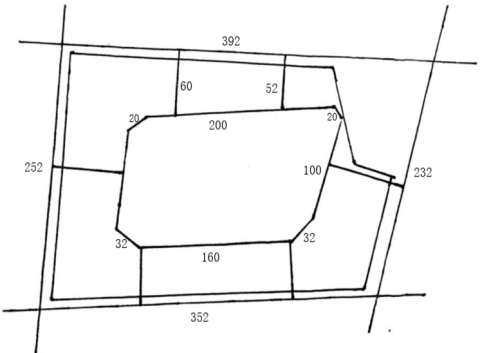
First, with the relevant length data captured, a road network map of the residential community was drawn, with annotations, as shown in Figure 2 (unit: m). In this map, there are 6 main intersections when the residential community is closed. According to the scale (1:2000) of the map, the distance of each connected road segment can be calculated, and with the Dijkstra algorithm, the shortest path Dij (i,j=1, 2, ..., 6) between every two points is obtained, as preparations for the distribution of traffic flow during the simulation below. With the above algorithm, the basic paths after the residential community is opened can also be obtained. Suppose the average speed υ of vehicles running around the residential community is 40km/h, then the average passing time of vehicles around the residential community can be obtained - $T=\frac{\Sigma_{i} \Sigma_{j} D_{i j}}{v}=755.34 \mathrm{s}$. After the residential community is opened, the number of main intersections is increased to 12. By the similar method, the average passing time of vehicles after the community is opened can be obtained, which is$T^{\prime}=\frac{\sum_{i} \Sigma_{j} D_{i j}}{v}=684.67 \mathrm{s}$. From a macro perspective, it can be seen that the average passing time of surrounding traffic after the residential community is opened is reduced.
Next, the software VISSIM was used to construct and simulate the road network of the residential community and its surrounding trunk roads. Since the residential community was closed at the moment, the roads within the residential community were disconnected from the external roads to indicate that vehicles from outside could not enter the residential community.
Figure 2. Road network map of Jiuzhou Xinshijie Huayuan
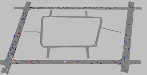
If a residential community is closed, none of the routes will pass through the residential community, so the traffic flow from outside the residential community were not allocated to the basic routes inside it. After the simulation program was run, with the default speed of the vehicles set to 40km/h, it could be clearly seen that the traffic volumes at intersections increased significantly, as shown in Figure 3.
Subsequently, observation points were set on each trunk road segment around the residential community to monitor and sample the traffic flow during the one-hour (7:30-8:30 a.m.) simulation, and the obtained data were analyzed and calculated. The calculation results of the proposed evaluation indicators mentioned in Section 2 are shown in Table 6.
Then, the residential community was opened. After simulation, it was found that, under the same conditions, the internal roads of the residential community shared part of the traffic outside the residential community after the residential community was opened, and that the traffic flow on the road segments improved significantly – the traffic volume per unit time was obviously improved, as shown in Figure 4.
Then, observation points were set on the trunk road segments at the same locations as above to monitor and sample the traffic flow during the one-hour simulation. The obtained data were analyzed and calculated, with the calculation results of each evaluation indicator shown in Table 7.
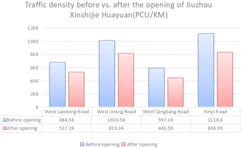
Through comparison of the changes in various evaluation indicators, it can be seen that the opening of the Type C residential community obviously improved the surrounding road traffic conditions. The differences between various indicators before and after opening are shown in Figure 5 and Figure 6.
Table 6. Statistics of the evaluation indicators for closed Jiuzhou Xinshijie Huayuan
|
Road segment |
West Laodong Road |
West Jinling Road |
West Qingliang Road |
Xinyi Road |
|
Traffic density (pcu/km) |
684.56 |
1016.58 |
597.16 |
1118.40 |
|
Road congestion rate (%) |
43.48 |
66.79 |
51.25 |
69.14 |
|
Road accessibility (%) |
52.91 |
55.29 |
50.28 |
51.63 |
|
Traffic delay time (s) |
62.55 |
|||
|
Number of intersection conflicts |
42.43 |
|||
|
Road segment |
West Laodong Road |
West Jinling Road |
West Qingliang Road |
Xinyi Road |
|
Traffic density (pcu/km) |
537.26 |
819.34 |
446.59 |
836.99 |
|
Road congestion rate (%) |
39.25 |
64.26 |
46.46 |
62.71 |
|
Road accessibility (%) |
56.34 |
58.29 |
61.03 |
54.33 |
|
Traffic delay time (s) |
41.10 |
|||
|
Number of intersection conflicts |
32.98 |
|||
Figure 4. Effect picture of Jiuzhou Xinshijie Huayuan after being opened
Figure 5. Comparison of traffic flow
Figure 6. Comparison of road congestion rates
3.3 Comparison model for open residential communities based on the grey relational algorithm
For the four types of open residential communities, this section uses the grey relational algorithm and combines quantitative and qualitative methods to make the original complex multi-factor comparison problem clearer and simpler and more convenient for calculation, and also to exclude the subjective arbitrariness of the observers to some extent. In this way, the effect relational grade sequence after the opening of the residential communities can be obtained objectively. In short, the grey relational grade analysis means that during the development of a system, if two factors change in the same way, that is, the degree of synchronous change is high, then the two factors can be considered as more related; otherwise, they are less related. Therefore, the grey relational analysis provides a way to quantitatively measure the development and change of a system, which is quite applicable to dynamic process analysis.
3.3.1 Overview of the grey relational algorithm
Grey relational analysis refers to the analysis of development trends based on the closeness of the sequence curve shapes of factors, and then provides some suggestions for decision makers [26]. The grey system theory puts forward the idea of performing grey relational analysis on each subsystem. The intention is to find out the numerical relationship between the subsystems (or factors) in the system by a certain method.
3.3.2 Specific steps of the grey relational algorithm
(1) Determine the comparison objects (evaluation target) and the reference sequence (evaluation criteria)
Suppose there are m evaluation objects and n evaluation indicators, the reference sequence is x0={x0(k)|k=1, 2, ..., n}, and the comparison sequence is xi={xi(k)|k=1, 2, ..., n}, i=1, 2, ..., m.
(2) Determine the weight of each indicator value
By such methods as AHP, the weights corresponding to each indicator $\varpi=\left[\varpi_{1}, \varpi_{2}, \dots, \varpi_{n}\right]$ can be obtained, where, ϖk, k=1, 2, ..., n, is the weight corresponding to the k-th evaluation indicator.
(3) Calculate the grey relational coefficient
$\xi_{i}(k)=\frac{\min _{s} \min _{t}\left|x_{0}(t)-x_{s}(t)\right|+\rho \max _{s} \tan \left|x_{0}(t)-x_{s}(t)\right|}{\left|x_{0}(k)-x_{i}(k)\right|+\rho \max _{s} \max _{t}\left|x_{0}(t)-x_{s}(t)\right|}$ is the relational coefficient of the comparison sequence xi to the reference sequence x0 on the k-th indicator, where $\rho \in[0,1]$ is the resolution coefficient [27]. In the formula, $\min _{s} \min _{t}\left|x_{0}(t)-x_{s}(t)\right|$ and $\max _{s} \max _{t}\left|x_{0}(t)-x_{s}(t)\right|$ are the two-stage minimum difference and the two-stage maximum difference, respectively. Generally speaking, the larger the resolution coefficient ρ, the greater the resolution; vice versa.
(4) Calculate the grey weighted relation
The calculation formula of the grey weighted relational grade is $r_{i}=\sum_{k=1}^{n} \varpi_{i} \xi_{i}(k)$, where ri is the grey weighted relational grade of the i-th evaluation object to the ideal object.
(5) Perform evaluation analysis
According to the magnitude of the grey weighted relational grade, the evaluation objects are sorted to form the relational sequence of evaluation objects. The greater the relational grade, the better the evaluation result.
3.3.3 Application of the grey relational algorithm in this study
Traffic density, traffic delay time and number of intersection conflicts are cost-based indicators while road congestion rate and road accessibility are efficiency-based indicators, and each indicator has a different dimension. In this paper, the changes in the above indicators are normalized, and the mean value method is adopted, that is, the value of each sequence is compared with the mean value of the entire line sequence. After normalization, the data of the comparison sequence and the reference sequence are shown in Table 8. The maximum value of the changes in each indicator is taken as the value of the virtual optimal residential community.
Let ρ=0.5, and calculate $\xi_{i}(k)$ and ri. The specific values of ri are listed in Table 9.
As shown in Table 9, the grey relational grade sequence is r3>r1>r2> r4; in other words, the surrounding road traffic is significantly improved for Type A and C residential communities after they are opened, followed by that of Type B residential communities, and that of Type D is not obviously improved.
Table 8. Values of the comparison sequence and the reference sequence
|
Evaluation indicator |
4 types of open residential communities |
Virtual optimal residential community |
|||
|
Type A |
Type B |
Type C |
Type D |
||
|
Traffic density (pcu/km) |
1.0806 |
0.8170 |
2.0012 |
0.1017 |
2.0012 |
|
Road congestion rate (%) |
1.4047 |
1.3721 |
1.1767 |
0.0465 |
1.4047 |
|
Road accessibility (%) |
0.8960 |
1.4109 |
1.4851 |
0.2030 |
1.4851 |
|
Traffic delay time (s) |
0.0034 |
0.2343 |
3.7500 |
0.0087 |
3.7500 |
|
Number of intersection conflicts |
0.7609 |
0.7885 |
2.1724 |
0.2805 |
2.1724 |
|
Type of residential community |
Type A |
Type B |
Type C |
Type D |
|
Grey weighted relational grade ri |
0.6130 |
0.4560 |
0.6527 |
0.0036 |
Based on the established vehicle traffic model, this paper employs the VISSIM traffic simulation technology to perform simulation test on a residential community, which directly shows the effect of traffic improvement after the residential community is opened. Through data analysis, the following conclusions are drawn: for residential communities with a large area and large traffic volume and those with a small area and large traffic volume, the surrounding road traffic is significantly reduced and the traffic pressure is greatly alleviated after the opening; the effect comes second for those with a large area and small traffic volume; and for those with a small area and small traffic volume, surrounding traffic sees no improvement. However, in this study, the impact of pedestrians on road traffic is deliberately ignored in the simulation. In fact, after a residential community is opened, pedestrians and vehicles will inevitably move in parallel in the residential community. Regarding this problem, a table of interference coefficients showing how pedestrians affect road traffic can be created and incorporated into the model. In addition, this study is also based on the assumption that there are no traffic lights at the intersections of the roads within the residential community. This assumption has some basis but cannot be applied to all circumstances. If the traffic in the residential community is too heavy, it will be necessary to set traffic lights. Traffic lights are a very important element in the construction of road networks, and their settings are also related to the types of intersections. Therefore, future research may take the types of intersections into account and add traffic lights in the scenarios to better simulate the actual situation after the opening of residential communities.
[1] Guegan, D.P., Martin, P.T., Cottrell, W.D. (2000). Prioritizing traffic-calming projects using the analytic hierarchy process. Transportation Research Record, 1708(1): 61-67. https://doi.org/10.3141/1708-07
[2] Gong, H.J., Li, B.C. (2006). Application of fuzzy comprehensive evaluation method in road transportation enterprises safety evaluation. Journal of Safety and Environment, 6(3): 54-57. https://doi.org/10.3969/j.issn.1009-6094.2006.03.017
[3] Chang, Z.Y., Sa, S.L., Fan, P.F. (2004). The first aid of urban accident based on GIS using AHP. Journal of Wuhan University of Technology, 28(2): 255-257. https://doi.org/10.3963/j.issn.2095-3844.2004.02.028
[4] Wang, E.M., Liu, X.J. (2007). Application of analytic hierarchy process and means of fuzzy comprehensive evaluating in choosing optimal plan of design about energy efficient residential buildings. Sichuan Building Science, 33(2): 146-149. https://doi.org/10.3969/j.issn.1008-1933.2007.02.040
[5] Wang, L.H., Zhang, Y. (2011). Application of the AHP and entropy weight method in evaluation on suitability of the urban construction land in Tianjin. Geological Survey and Research, 34(4): 305-312. https://doi.org/10.3969/j.issn.1672-4135.2011.04.009
[6] Yu, J.F., Li, W., Gong, X.L. (2013). Study on the status evaluation of urban road intersections traffic congestion base on AHP-TOPSIS modal. Procedia - Social and Behavioral Sciences, 96: 609-616. https://doi.org/10.1016/j.sbspro.2013.08.071
[7] Nosal, K., Soleck, K. (2014). Application of AHP method for multi-criteria evaluation of variants of the integration of urban public transport. Transportation Research Procedia, 3: 269-278. https://doi.org/10.1016/j.trpro.2014.10.006
[8] Żak, J., Kruszyński, M. (2015). Application of AHP and ELECTRE III/IV methods to multiple level, multiple criteria evaluation of urban transportation projects. Transportation Research Procedia, 10: 820-830. https://doi.org/10.1016/j.trpro.2015.09.035
[9] Barić, D., Pilko, H., Strujić, J. (2016). An analytic hierarchy process model to evaluate road section design. Transport, 31(3): 312-321. https://doi.org/10.3846/16484142.2016.1157830
[10] Li, H.M., Ni, F.J., Dong, Q., Zhui, Y.Q. (2018). Application of analytic hierarchy process in network level pavement maintenance decision-making. International Journal of Pavement Research and Technology, 11(4): 345-354. https://doi.org/10.1016/j.ijprt.2017.09.015
[11] Mei, X.B., Wang, F.G., Cao, J.F. (2000). The application of fuzzy comprehensive evaluation on water quality and discussion. World Geology, 19(2): 172-177.
[12] Yu, K.L., Yang, Y.S., Zhang, C.P. (2007). Application of fuzzy comprehensive evaluation method in identifying water source of water-rush in underground shaft. Metal Mine, (3): 47-50. https://doi.org/10.3321/j.issn:1001-1250.2007.03.013
[13] Wang, X., Huo, D.L. (2008). Application of fuzzy comprehensive evaluation in coal safety assessment. China Mining Magazine, 17(5): 75-78. https://doi.org/10.3969/j.issn.1004-4051.2008.05.022
[14] Shao, H.Y., Liu, Q., Li, X.L. (2006). Application of AHP in designing of wastewater treatment plant. Environmental Science & Technology, 29(2): 98-100. https://doi.org/10.3969/j.issn.1003-6504.2006.02.040
[15] Yang, H.Z., Kang, F.J., Li, J. (2002). The application of AHP in integrative process of assessing the credibility of underwater vehicle system simulation. Acta Simulata Systematica Sinica, 14(10): 1299-1301. https://doi.org/10.3969/j.issn.1004-731X.2002.10.010
[16] Mogridge, M.J. (1997). The self-defeating nature of urban road capacity policy: A review of theories, disputes and available evidence. Transport Policy, 4(1): 5-23. https://doi.org/10.1016/S0967-070X(96)00030-3
[17] Rossi, G., Lombardi, M., Mascio, P.D. (2018). Consistency and stability of risk indicators: The case of road infrastructures. International Journal of Safety and Security Engineering, 8(1): 39-47. https://doi.org/10.2495/SAFE-V8-N1-39-47
[18] Yang, X.G., Lao, Y.T., Yun, M.P. (2007). Application of different pedestrian cross pattern to no-signal controlled segment. Journal of Tongji University, 35(11): 1466-1469. https://doi.org/10.3321/j.issn:0253-374X.2007.11.005
[19] Siregar, M.L., Agah, H.R., Hidayatullah, F. (2018). Near-miss accident analysis for traffic safety improvement at a ‘channelized’ junction with u-turn. International Journal of Safety and Security Engineering, 8(1): 31-38. https://doi.org/10.2495/SAFE-V8-N1-31-38
[20] Ziegelmeyer, A., Koessler, F., My, K.B., Denant-Boèmont, L. (2008). Road traffic congestion and public information: An experimental investigation. Journal of Transport Economics and Policy, 42(1): 43-82.
[21] Olsson, J. (2009). Improved road accessibility and indirect development effects: Evidence from rural Philippines. Journal of Transport Geography, 17(6): 476-483.
[22] Du, H.B., Mulley, C. (2006). Relationship between transport accessibility and land value: Local model approach with geographically weighted regression. Transportation Research Record, 1977(1): 197-205. https://doi.org/10.1177/0361198106197700123
[23] Lu, T.C., Kang, K. (2009). The application of entropy method and AHP in weight determining. Computer Programming Skills & Maintenance, (22): 19-22. https://doi.org/10.3969/j.issn.1006-4052.2009.22.009
[24] Feng, S., Li, L.D. (1999). Decision support for fuzzy comprehensive evaluation of urban development. Fuzzy Sets and Systems, 105(1): 1-12. https://doi.org/10.1016/S0165-0114(97)00229-7
[25] Wang, Y., Yang, W.F., Li, M., Liu, X. (2012). Risk assessment of floor water inrush in coal mines based on secondary fuzzy comprehensive evaluation. International Journal of Rock Mechanics and Mining Sciences, 52: 50-55. https://doi.org/10.1016/j.ijrmms.2012.03.006
[26] Kuo, Y., Yang, T., Huang, G.W. (2008). The use of grey relational analysis in solving multiple attribute decision-making problems. Computers & Industrial Engineering, 55(1): 80-93. https://doi.org/10.1016/j.cie.2007.12.002
[27] Singh, P.N., Raghukandan, K., Pai, B.C. (2004). Optimization by grey relational analysis of EDM parameters on machining Al-10%SiCP composites. Journal of Materials Processing Technology, 155-156: 1658-1661. https://doi.org/10.1016/j.jmatprotec.2004.04.322