Kalpana Polisetty* | Kiran Kumar Paidipati | Jyostna Devi Bodapati
OPEN ACCESS
Rainfall forecast is a hotspot in meteorological studies in the last few years. The key difficulty in forecast accuracy lies in the nonlinearity of rainfall data. Considering the potential of support vector machine (SVM) to solve nonlinear time series, this paper develops an SVM-based model based on the monthly rainfall data from 1901 to 2015 in Northwest India. The forecast accuracies of four different kernels were compared, including linear, polynomial, radial basis function (RBF) and sigmoid kernels. The comparison shows that the SVM-based model with the RBF kernel achieved the smallest root mean squared error (RMSE) at the lookback of 25, C=1, γ =0.01 and =0.1. Our research provides an effective tool to predict rainfall in regions with similar meteorological conditions to northwest India.
support vector machine (SVM), kernels, rainfall forecast, accuracy, northwest India
The meteorological variables like rainfall, temperature, humidity, evaporation, etc. exhibit high levels of stochasticity and make predictions over time quite challenging. Rainfall and its accurate prediction are very essential for agronomic countries like India. Historically, records of extreme rainfall patterns have been experienced in India. For example, in some parts of North-West India had often witnessed massive rainfalls leading to floods, as well as, droughts and famines due to limited rainfall. An important issue is to monitor closely the rainfall variations across the country on both temporal and spatial scale. Farmers solely rely on rainfall water for providing crops with the water requirements during both wet and semi-wet weather conditions. To maintain a balanced living and economy of the country, requires an analysis of rainfall to understand the optimal patterns of rainfall behaviour which could be complex and non-linear in nature. Automatic prediction of the rainfall patterns is a key factor to observe the nature of Indian rainfall and would require advanced forecasting models. Therefore, it is very significant to model, forecast and monitor rainfall in the agricultural actions [1].
The examination of the accuracy in forecasting models is a fundamental aspect in many decision processes [2]. The main aim of forecasting is to observe and build model for the available input, in order to estimate the unknown value of future data accurately. In recent times, forecasting of time series data is an active research area in water resources management [3]. In finding solutions for hydrological issues, many researchers have applied time series theories and techniques [4]. Generally, identifying and solving hydrological problems are burning issues due to several anthropogenic and other natural factors [5]. The support vector machine (SVM) was first introduced by Vapnik and it was mainly developed for regression estimation problems, solving pattern recognition, data mining, classification, and especially time series prediction [6-8]. In addition to classification, SVM can also be used for regression. Support vector regression (SVR) has become most popular in the recent past due its ability to solve more complex classification and prediction problems [9]. The ability of SVR to model complex nonlinear data for regression makes SVR popular. Similar to SVM, SVR is also designed to model linear data. But with the introduction of kernel functions, SVR is able to model complex non-linear structures in the data [7]. SVR is a robust model to predict the data like rainfall, temperature which are highly complex in nature. In hydrology and associated areas, the SVM models are applied for hydrological predictions [10-15]. Other than that, Lin et al. [11] used SVM to predict reservoir inflow during typhoon-warning period, Misra et al. [16] used SVM to simulate runoff and sediment yield from watershed with monsoon period data.
The SVM has been more often used by the above cited researchers to forecast the time series problems in various fields. Therefore, the aim of this study is to investigate the historical behaviour of the monthly rainfall in India, particularly in the North-West region. The research problem in this paper involves the applicability of the SVM model and its ability to forecast the rainfall time series data. Other than that, this research will focus on the application of several kernel functions in SVM and the effect of changing the kernel functions will be evaluated as well.
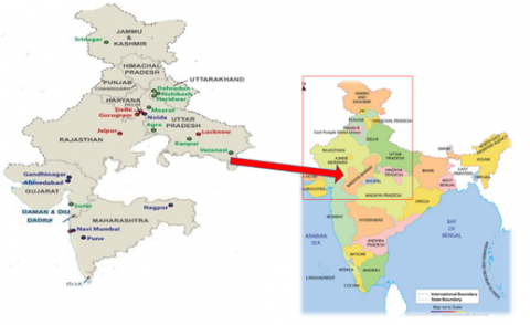
In this study, monthly rainfall data is collected from Open Government Data (OGD) platform India. The data is collected for the duration of 115 years from January 1901 to December 2015 bringing 1380 observations. Most of the people in the north side of India consume wheat as primary food and the North-West of India is the region for the production of the wheat and is also called as ‘wheat bowl’ of the country [17]. The 69◦-85◦ E longitudes and 23◦-37◦ N latitudes are the approximate boundaries in the south Asia which occupy the landmass of around 1,010,654 km2 in the North-West India. The region of the North-West consists of 9 meteorological subdivisions of India. The location of the catchment areas are illustrated in Figure 1.
Figure 1. The location of catchment area in the North-West India
2.1 Forecasting models
This section discusses about in details regarding SVM and the choice of kernels used in this study. Kernel functions are required to use with SVM when the data is more non-linear. These kernels are helpful to project the data from its original space to a new space where the data can be well separated. We have applied all the 4 default kernels to project the data. These kernels are much widely used for many applications. In the Recent years, the applications of SVM have been rapidly grown for solving classification and regression problems. The SVM has the capability to develop complex nonlinear relationship models with the help of well suited kernel function. Basically, SVM can be applied to classification and regression problems. In case of classification problems, the given test sample has to be assigned to one of the given finite set of classes. The number of classes is finite and usually varies from 10s to 100s. In case of the regression models, a continuous value has to be predicted given a test data sample. Classification is a specific case of regression problems. SVR stands for support vector based regression that uses a different loss function that is quadratic and Hinge loss functions. The given data is partitioned into training and test sets. Let the training set of ‘n’ data points {xi, yi}n i=1 where xiÎRp (P is the dimension of the data in the original space) and yiÎR, is the value to be predicted and can be achieved using the following:
$y=f(x)=w^{T} \varphi(x)+b$ (1)
where, φ(x) is the representation of the given data sample x in the high dimensional feature spaces. The transformation from the original space x to the projected space φ(x) is non-linearly mapped [18]. Cost function of SVM can be represented as the following minimization function assuming w and b as the parameters that are to be estimated:
$\min J(w, e)=\frac{1}{2} w^{T} w+C \sum_{i=1}^{n}\left(\xi_{k}+\xi_{k}^{*}\right)$ (2)
Subject to the constraints:
$y_{k}-w^{T} \varphi\left(x_{k}\right)-b \leq \varepsilon+\xi_{k}$
$w^{T} \varphi\left(x_{k}\right)+b-y_{k}-\leq \varepsilon+\xi_{k}^{*}$
$\xi_{k}^{*}, \xi_{k} \geq 0$
The objective function is the sum of two parts. The first part $(1 / 2)\|w\|^{2}$ represents the norm of the weight vector w and the second part of the function acts as regularizer and C is referred to as the regularizing constant. This parameter C determines to which part of the objective function weightage has to be given that is either to the empirical error or to the regularization term. In case of SVR, a new parameter ‘ε’ is introduced that represents the size of the tube. Here, ξ and ξ* are the slack variables. Now the objective function can have the following explicit form:
$y(\mathbf{x})=\sum_{i=1}^{n}\left(a_{i}-a_{i}^{*}\right) K\left(\mathbf{x}_{i}, \mathbf{x}_{j}\right)+b$ (3)
In Eq. (3), $a_{i}$ and $a_{i}^{*}$ are assigned as Lagrange multipliers. They satisfy the equalities $a_{i} * a_{i}^{*}=0, a_{i} \geq 0,$ and $a_{i}^{*} \geq 0$ where i=1,2,..., n and these are obtained by maximizing the dual function which has the following form:
$\operatorname{Max} \mathrm{R}\left(\mathrm{a}_{\mathrm{i}}, \mathrm{a}_{\mathrm{i}}^{*}\right)=\sum_{i=1}^{n} d_{i}\left(a_{i}-a_{i}^{*}\right)-\varepsilon \sum_{i=1}^{n}\left(a_{i}+a_{i}^{*}\right)$
$-\frac{1}{2} \sum_{i=1}^{n} \sum_{j=1}^{n}\left(a_{i}-a_{i}\right)\left(a_{j}-a_{j}^{*}\right) K\left(x_{i}, x_{j}\right)$ (4)
Subject to the constraints:
$\sum_{i=1}^{n} a_{i}=\sum_{i=1}^{n} a_{i}^{*}, 0 \leq a_{i} \leq C$ and $0 \leq a_{i}^{*} \leq C$ for $i=1,2, \ldots, n$
The kernel function, $K\left(\mathbf{x}_{i}, \mathbf{x}_{j}\right)$ can be expressed as the inner product:
$K\left(\mathbf{x}_{i}, \mathbf{x}_{j}\right)$ (5)
Another important term is kernel, it plays vital role in SVM. There are various types of kernels that are supported with the support vector machines models. These kernels include linear, polynomial, radial basis function (RBF), sigmoid etc. The kernel functions are defined as:
Table 1. Different types of Kernel functions
|
Kernel |
Formula |
Parameters |
|
Linear |
$\mathrm{x}_{\mathrm{i}}^{*} \mathrm{y}_{\mathrm{i}}$ |
C and γ |
|
Polynomial |
$\left(\gamma_{\mathbf{X}_{\mathbf{i}}} \mathbf{x}_{\mathbf{j}}+\mathbf{r}\right)^{d}$ |
C, γ, r and d |
|
RBF |
$\exp \left(-\gamma\left|\mathrm{x}_{\mathrm{i}}-\mathrm{x}_{\mathrm{j}}\right|^{2}\right)$ |
C and γ |
|
Sigmoid |
$\tanh \left(\gamma \mathrm{X}_{\mathrm{i}} \mathrm{X}_{\mathrm{j}}+\mathrm{r}\right)$ |
C, γ, r |
Explanation- C: cost; γ: gamma; r: coefficient; d: degree.
where, the basic form of kernel function is $K\left(x_{i}, \mathrm{x}_{j}\right)=\varphi\left(x_{i}\right)^{T} \times \varphi\left(x_{j}\right)$, it represents the product of input data points mapped into the higher dimensional feature space by transformation function ϕ [12,18-20]. Root Mean Square Error (RMSE) is used as the performance measure to evaluate the proposed model. That is the model with the lesser RMSE is considered to be the better model than other models. The RMSE is defined as follows:
$\mathrm{RMSE}=\sqrt{\frac{1}{n} \sum_{t=1}^{n}\left(y_{t}-\hat{o}_{t}\right)^{2}}$ (6)
where, $y_{t}$ is the actual value and $\hat{o}_{t}$ is the predicted at the time t.
The core objective of this work is to build a better forecasting model by using SVM and also comparing various SVM kernel functions like Linear, Polynomial, RBF and Sigmoid on the prediction task. Till date which type of kernel is decided empirically and selection of the type of kernel is an active area of research. We use 115 years rainfall data to understand the efficiency of the proposed model. The data is divided into train and test sets in the ratio of 80:20 proportion. The train set contains 1104 observations starting from January 1901 to December 1993, while the test set contains 276 points, from January 1994 to December 2015.
Training data is used only for development of model and testing data is considered to examine the performance of the model on untrained data. We have tried a method called look back that uses the previous 25 months data to predict the current month rainfall. The analysis initially started with selection of look back values and the performance of training and testing data for various look back orders is shown in Table 2.
Table 2. Performance of the model with different kernels with different look back values
|
Kernel |
Look Back |
Train RMSE |
Test RMSE |
|
Linear |
5 |
48.78 |
48.30 |
|
10 |
34.37 |
34.57 |
|
|
15 |
26.95 |
29.66 |
|
|
20 |
26.69 |
29.22 |
|
|
25 |
24.48 |
26.54 |
|
|
RBF |
5 |
27.83 |
30.75 |
|
10 |
23.79 |
26.28 |
|
|
15 |
18.42 |
29.02 |
|
|
20 |
21.07 |
27.21 |
|
|
25 |
22.54 |
24.81 |
|
|
Sigmoid |
5 |
50.12 |
49.04 |
|
10 |
35.14 |
34.59 |
|
|
15 |
28.98 |
30.95 |
|
|
20 |
26.98 |
28.30 |
|
|
25 |
24.96 |
25.47 |
|
|
Polynomial |
5 |
64.34 |
62.53 |
|
10 |
32.35 |
33.75 |
|
|
15 |
24.78 |
31.39 |
|
|
20 |
22.49 |
30.07 |
|
|
25 |
19.3 |
27.68 |
Table 3. Performance of RBF kernel function with look back=25, various C and γ values
|
C |
γ |
Train RMSE |
Test RMSE |
|
1 |
0.01 |
22.54 |
24.81 |
|
2 |
0.02 |
21.70 |
24.91 |
|
3 |
0.03 |
20.95 |
25.04 |
|
4 |
0.04 |
19.93 |
25.36 |
|
5 |
0.05 |
18.77 |
25.88 |
|
6 |
0.06 |
17.64 |
26.46 |
|
7 |
0.07 |
16.48 |
26.88 |
|
8 |
0.08 |
15.15 |
27.32 |
|
9 |
0.09 |
13.80 |
27.74 |
Based on Table 3, it is evident that the RBF is more accurate than the other kernels at the look-back of 25. Normally, it is irrational to make a judgement based on the look-back only, but this study must select a particular look-back value. In subsequent analysis, the look-back was fixed at 25, while the C-value and Gamma were changed constantly. Then, it is observed that the RMSE of the training data decreased, while that of the testing data increased. At C=1 and γ=0.01, it is observed that the data has less error compared to remaining set of values of C and γ. So the decision is taken as C=1 and γ=0.01 are the appropriate parameters in this phase.
Table 4. Performance of RBF kernel function with look back =25, C =1 and various γ values
|
γ |
Train RMSE |
Test RMSE |
|
0.0001 |
40.22 |
37.12 |
|
0.0005 |
26.77 |
26.37 |
|
0.001 |
25.05 |
25.43 |
|
0.002 |
24.15 |
25.07 |
|
0.005 |
23.16 |
24.82 |
|
0.01 |
22.54 |
24.81 |
|
0.02 |
21.97 |
24.88 |
|
0.05 |
21.02 |
25.32 |
|
0.1 |
19.43 |
25.93 |
|
0.5 |
12.62 |
31.77 |
|
1 |
11.52 |
42.11 |
|
5 |
39.16 |
86.79 |
|
10 |
40.63 |
88.12 |
|
100 |
40.67 |
88.15 |
|
ε |
Train RMSE |
Test RMSE |
|
0.001 |
22.58 |
24.87 |
|
0.005 |
22.58 |
24.84 |
|
0.01 |
22.57 |
24.82 |
|
0.05 |
22.54 |
24.81 |
|
0.1 |
22.53 |
24.81 |
|
0.2 |
22.84 |
24.94 |
|
0.3 |
24.21 |
26.01 |
|
0.4 |
26.40 |
27.95 |
|
0.5 |
29.34 |
31.13 |
|
0.6 |
35.01 |
36.60 |
|
0.7 |
41.51 |
42.96 |
|
0.8 |
48.76 |
49.89 |
|
0.9 |
55.75 |
56.61 |
From the Table 4, the look back and C values are fixed at particular point, then the set of Gamma values are considered for RBF kernel to study the error patterns. When the gamma values are changes as increasing or decreasing, the RMSE values could not follow any pattern. However, the optimum gamma value is identified as 0.01 from the Table 4.
Table 6. Summarized results of various kernels with optimum parameters
|
Kernel |
Look Back |
C |
γ |
ε |
Train RMSE |
Test RMSE |
|
Linear |
25 |
9 |
0.9 |
0.1 |
24.47 |
26.54 |
|
Polynomial |
25 |
1 |
0.1 |
0.1 |
19.30 |
27.68 |
|
RBF |
25 |
1 |
0.01 |
0.1 |
22.54 |
24.81 |
|
Sigmoid |
25 |
2 |
0.0006 |
0.1 |
24.96 |
25.47 |
Finally, the look back, C, γ values are fixed at 25, 1, 0.01 and the various epsilon values are considered from 0.001 to 0.9. The analysis exhibits ε=0.001 to 0.1, the RMSE values for train and test are decreased and ε=0.2 to 0.9, the RMSE values for training and testing are increased. Here, it is observed that ε=0.1 shows lowest error and it is identified as best parameter. However, the SVM analysis exhibits look back=25, C=1, g=0.01 and e=0.1.
The same procedure i.e., trial and error methods are continued to examine the remaining kernels i.e., linear, polynomial and sigmoid. The summarized results are presented in the Table 6. From the Table 6, the individual kernels obtained the best parameters and lowest RMSE values are linear kernel shows look back=25, C=9, γ=0.9, ε=0.1 and RMSE values (24.47, 26.54); polynomial kernel given look back=25, C=1, γ=0.1, ε=0.1 and RMSE values (19.30, 27.68); RBF obtained look back=25, C=1, γ=0.01, ε=0.1 and RMSE values (24.81, 24.81) and sigmoid kernel shows look back=25, C=2, γ=0.0006, ε=0.1 and RMSE values (24.96, 25.47).In this experiment, the best performance is achieved using RBF kernel with parameters look back=25, C=1, γ=0.01, ε=0.1. The performance of RBF model is outperformed when compared with other kernels. Therefore, RBF kernel with parameters C=1, γ=0.01, ε=0.1 are well suits to build the accurate model and forecast to monthly rainfall patterns.
This study set out with the aim of assessing the application of SVM in forecasting rainfall data in the North-West India. Several type of kernels functions such as linear, polynomial, RBF and Person are applied to develop adequate time series models. The current study found that only RBF kernel has fitted exactly to forecast the rainfalls of Northwest India. This experiment shows how the RBF kernel performs very well on considered Northwest rainfall data and learning tasks. The accuracy of the models was compared based on measurement statistic RMSE.
[1] Hoogenboom, G. (2000). Contribution of agromete-orology to the simulation of crop production and its applications. Agricultural Forest Meteorology, 103(1-2): 137-157. https://doi.org/10.1016/S0168-1923(00)00108-8
[2] Zhang, G.P. (2003). Time series forecasting using a hybrid ARIMA and neural network model. Neurocomputing, 50: 159-175. https://doi.org/10.1016/S0925-2312(01)00702-0
[3] Huang, W., Bing, X. B., Hilton, A. (2004). Forecasting flow in apalachicola river using neural networks. Hydrological Processes, 18(13): 2545-2564. https://doi.org/10.1002/hyp.1492
[4] Lin, G.F., Lee, F.C. (1992). An aggregation-disaggregation approach for hydrologic time series modelling. Journal of Hydrology, 138(3-4): 543-557. https://doi.org/10.1016/0022-1694(92)90136-J
[5] Kim, S.J., Hyun, Y., Lee, K.K. (2005). Time series modeling for evaluation of groundwater discharge rates into an urban subway system. Geosciences Journal, 9(1): 15-22. https://doi.org/10.1007/BF02910550
[6] Smola, A.J., Scholkopf, B. (2004). A Tutorial on support vector regression. Statistics and Computing, 14(3): 199-222. https://doi.org/10.1023/B:STCO.0000035301.49549.88
[7] Tay, F.E.H., Cao, L.J. (2001). Improved financial time series forecasting by combining support vector machines with self-organizing feature map. Intelligent Data Analysis, 5(4): 339-354. https://doi.org/10.3233/IDA-2001-5405
[8] Vapnik, V. (1995). The Nature of Statistical Learning Theory. Springer Verlag, Berlin.
[9] Ismail, S., Shabri, A. (2014). Time series forecasting using least square support vector machine for Canadian Lynx Data. Jurnal Teknologi, 70(5): 11-15. https://doi.org/10.11113/jt.v70.3510
[10] Asefa, T., Kemblowski, M., Mckee, M., Khalil, A. (2006). Multi-time scale streamflow predictions: the support vector machines approach. Journal of Hydrology, 318(1-4): 7-16. https://doi.org/10.1016/j.jhydrol.2005.06.001
[11] Lin, J.Y., Cheng, C.T., Chau, K.K. (2006). Using support vector machines for long-term discharge prediction. Hydrological Sciences Journal, 51(4): 599-612. https://doi.org/10.1623/hysj.51.4.599
[12] Maity, R., Bhagwat, P.P., &Bhatnagar, A. (2010). Potential of support vector regression for prediction of monthly streamflow using endogenous property. Hydrological Processes, 24: 917-923. https://doi.org/10.1002/hyp.7535
[13] Dibike, Y.B., Solomatine, D.P. (2001). River flow forecasting using artificial neural networks. Physics and Chemistry of the Earth, Part B: Hydrology. Oceans and Atmosphere, 26(1): 1-7. https://doi.org/10.1016/S1464-1909(01)85005-X
[14] Elshorbagy, A., Corzo, G., Srinivasalu, S., Solomantine, D.P. (2010a). Experimental investigation of the predictive capabilities of data driven modeling techniques in hydrology - Part 1: Concepts and methodology. Hydrology and Earth System Sciences, 14(10): 1931-1941. https://doi.org/10.5194/hess-14-1931-2010
[15] Elshorbagy, A., Corzo, G., Srinivasalu, S., Solomantine, D.P. (2010b). Experimental investigation of the predictive capabilities of data driven modeling techniques in hydrology - Part 2: Application. Hydrology and Earth System Sciences, 14(10): 1943-1961. https://doi.org/10.5194/hess-14-1943-2010
[16] Misra, D., Oommen, T., Agarwal, A., Mishra, S.K., Thompson, A.M. (2009). Application and analysis of support vector machine based simulation for runoff and sediment yield. Biosystems Engineering, 103(4): 527-535. https://doi.org/10.1016/j.biosystemseng.2009.04.017
[17] Yadav, R.K., Rupa, K.K., Rajeevan, M. (2012). Characteristic features of winter precipitation and its variability over northwest India. Journal of Earth System Science, 21(3): 611-623. https://doi.org/10.1007/s12040-012-0184-8
[18] Thomas, H., Lewicki, P. (2006). Statistics: methods and applications. StatSoft, United Kingdom.
[19] Karin, K. (2012). A Comparison of various forecasting methods for auto correlated time series. International Journal of Engineering Business Management, 4: 1-6. https://doi.org/10.5772/51088
[20] Veeranjaneyulu, N., Sujatha, V., Devi, B.R. (2014). Scene Classification Using Support Vector Machines With LDA. Journal of Theoretical & Applied Information Technology. https://doi.org/10.1109/ICACCCT.2014.7019421