Junzhen Meng* | Junran Zhang
OPEN ACCESS
The purpose of this study was to investigate the generation of non-overlapping particle sets quickly and accurately that meet specified conditions in the preparatory stage of discrete element simulation. A fast-geometric particle stackinfg algorithm based on geometric and grid search method was proposed for the generation of particle stacking, which is used to generate large particles, then generated small particles and fill them. The results indicated when the velocity of particle generation was too slow, the new position of two or three contacts should be adjusted to accommodate more particles in the current particle diameter range. Moreover, the calculation example showed that under the condition of a specified particle gradation, particle sets with different void ratios could be generated according to the need for discrete element simulation. The time to generate the particle sets is linear with the number of particles, and the algorithm takes less time. The findings of this study may serve as the generation of non-overlapping particle sets for meeting specified conditions in discrete element simulation.
particle packing, fast particle random algorithm, discrete element, 2D/3D generation efficiency
In the preliminary preparation stage of discrete element simulation [1-5], complementary and crossed particle set must be generated rapidly in the designated area, namely, particle accumulation. The stacking algorithm is mainly divided into two categories. One is the dynamic method [6-8], such as gravity deposition [9-11], expansion method [12-14] and compression method [15-17]. The main principle of discrete element calculation on initially generated particles set is according to Newton's motion law of overlapping particles to recalculate the new location, until mutually overlap between particles, however, due to real-time dynamic contact detection requires 60 % ~ 70 % of the time, using PFC2D/3D generated tens of thousands to hundreds of thousands of particles is very time consuming, needs many days to get the results. However, the particle density can reach more than 0.60 based on the physical principle. The other is the construction method [2, 18-22] which is based on the pure geometric algorithm. The radius and position of particles are determined through geometric calculation without involving mechanical calculation. The calculation amount of boundary retrieval is greatly decreased and the generation speed is much faster than that of the dynamic method. However, the density of particle deposition is relatively low, generally between 0.5 and 0.57. The construction method also has some shortcomings. The gradation of particles cannot be well reflected, most of which are randomly distributed within a certain size range. It is feasible for some materials, but accurate gradation information of particles should be considered for soil materials. The density of the directly generated particle set is relatively fixed within the specified particle range or under the specified gradation, so it cannot be adjusted and controlled well according to the requirements of the simulation material properties, and the function can be achieved is single.
In the geotechnical field, especially in soil mechanics, such as landslide, debris flow, and laboratory triaxial simulation, it is of great significance to rapidly generate particle sets with certain gradation and porosity ratio, which provides a basis for further discrete element simulation analysis of geotechnical engineering problems. Therefore, it is urgent to have a new algorithm that can not only generate the model with the specified density but also generate it quickly when the gradation is fixed. This paper includes four parts, the introduction, the fast particle random algorithm, the algorithm efficiency and the result analysis and the conclusion.
Figure 1. The schematic process of particle generation
There are many methods to fill a cup with as many balls of different radii as possible. These methods generally fall into two categories: Filling small balls before large ones (small ball-first strategy), and filling large balls before small ones (large ball-first strategy). The latter strategy brings relatively high density of balls in the cup. Therefore, this paper designs an algorithm based on the large ball-first strategy. The particle generation is shown in Figure 1.
Figure 2. Main program algorithmic flow chart
Figure 3. Subprogram flow chart
In the generated ball, it needs to verify with the adjacent balls whether it has an intersection with the current balls, and the retrieval of adjacent particles is very time-consuming. Therefore, according to the characteristics of the algorithm, the grid method is selected. To prevent large particles from crossing the adjacent grid area, the ratio between the maximum particle radius and the lattice interval needs to be set, and the ratio needs to be greater than two.
Like other fast stacking algorithms, there may be no room for more particles in the later stage if the current particle stacking position is not adjusted. Therefore, the current particle position needs to be adjusted in a certain stage of generation. In the classical stacking process, if there is an intersection between particles, which can be calculated using Newton's equation of motion, but the time cost is high, and the algorithm is tangent between aggregate particles, even given physical parameters do not produce force. Therefore, the micro-adjustment of the ball within a certain range is adopted to provide a greater probability for the generation of new particles in the later stage. The algorithm is implemented in MATLAB 2014a environment, and the specific process is shown in Figure 2 and Figure 3 above.
Description:
(1) Parameter settings including the sample void ratio e, gradation, the fluctuation range of different particle radius(rang), the sample generation area (X, Y, Z), the grid spacing and maximum particle radius ratio gid, the search radius index corresponding to the radius of each particle af, the number of reshape.
(2) The range of fluctuations for different particle radii is 0 to 1, and the particles are selected according to the radius. The radius is usually 0.1 to 0.4, The formula is
$r^{\prime}=r(1+2(\operatorname{rand}-0.5) \cdot \operatorname{rang})$ (1)
where, the $r^{\prime}$ is the radius after change, random numbers with rand 0 to 1.
(3) The search radius index af is the retrieval distance range between balli and surrounding ballnp in the gradation group j: [ri+rnp+2rnew×afj,1, ri+rnp+2rnew×afj,2], where, afj,2>afj,1. Due to the prevention of excessive aggregation of large particles during the initial generation of large particles, generally the larger the balls are, the larger the af are. When the particle radius is small, to prevent the retrieval calculation amount and the spacing between small particles to be too large, af can be set to be smaller.
(4) Mesh the sample generation area, and each grid corresponds to a cell matrix, which is used to store balls whose center position is within the scope of this space.
(5) Random position completely, the coordinate (x, y, z) within the scope of cell space, which is generated randomly.
(6) Random position of contact. Contact with the random position within a certain range of the currently generated nuclear ball:
$(x, y, z)_{n e w}=(x, y, z)_{b a l l}+\left(r_{b a l l}+r_{n e w}\left(1+r a n d_{1 \times 3}\right)\right) \cdot \overrightarrow{d i r}$ (2)
where, (x, y, z) is the coordinate, r is the radius, rand1×3$\in$[0,1] is the unit random vector, and $\overrightarrow{d \iota r}$ is the unit random vector.
(7) The double contact is generated randomly. In the three-dimensional space, for two balls that are adjacent to each other, the distance equation between one point and two balls in the space is
$\left\{\begin{array}{l}{\left(x-x_{A}\right)^{2}+\left(y-y_{A}\right)^{2}+\left(z-z_{A}\right)^{2}=\left(r+r_{A}\right)^{2}} \\ {\left(x-x_{B}\right)^{2}+\left(y-y_{B}\right)^{2}+\left(z-z_{B}\right)^{2}=\left(r+r_{B}\right)^{2}}\end{array}\right.$ (3)
Since the Eq. (3) has an infinite number of solutions, its value can be limited by the following formula
$z=z_{A}+r a n d \cdot\left(z_{B}-z_{A}\right)$ (4)
In this way, two solutions can be obtained.
(8) Three-contact generation is obtained by the Eq. (5)
$\left\{\begin{array}{l}{\left(x-x_{A}\right)^{2}+\left(y-y_{A}\right)^{2}+\left(z-z_{A}\right)^{2}=\left(r+r_{A}\right)^{2}} \\ {\left(x-x_{B}\right)^{2}+\left(y-y_{B}\right)^{2}+\left(z-z_{B}\right)^{2}=\left(r+r_{B}\right)^{2}} \\ {\left(x-x_{C}\right)^{2}+\left(y-y_{C}\right)^{2}+\left(z-z_{C}\right)^{2}=\left(r+r_{C}\right)^{2}}\end{array}\right.$ (5)
(9) To get a solution of an equation you have to get rid of the plurality solution, and the sequence of post-screening is, complete random position, contact random position, double contact random position, three contact position, and try to highlight the nature of random generation, otherwise it is easy for some balls to be excessively clustered and deviate from the reality.
(10) In the two-dimensional particle accumulation simulation, there is no three-contact generation, because in two-dimensional, two equations can directly calculate two accurate solutions.
(11) Reshape subroutine is shown in Figure 3, select balls within the diameter range of the ball adjacent to the ball itself, and select three of them to calculate the three contact positions. If the current particle does not have any cross, it is correct Dynamic systems in Newton's laws of motion, ‘arch’ can be formed in the process of dynamically generated. it is possible to limit other particles in the space-filling, reduce the particle packing density. It is not based on physics principle Reshape function, only relying on pure geometric properties, can effectively avoid this problem.
3.1 2D generation efficiency
Concerning literature [23], it was generated in the finger region. The gradation was selected as 0.029 cm to 0.2cm(rmax/rmin=7) in the first group and 0.1cm to 0.2 cm (rmax/rmin=2) in the second group. The gradation was evenly distributed. The remaining parameters of the model are set as shown in Table 1. The results of the particle set under different gradations are shown in Figures 4-7.
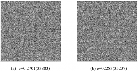
It can be seen from the Figure 4-7, under the same gradation model can obtain different void ratio deposit of particles, the particle packing density under the first set of grading can be in 0.826 to 0.860 (void ratio e is 0.163 to 0.211, the packing density of ρ=1/(1+e)), the second set of densities can be in 0.787 to 0.814 (void ratio e is 0.229 to 0.271), but with the decrease of the void ratio, density increase, model generation time is gradually enlarged. As the void ratio decreases, it takes more time to fill the current particle with more particles and to adjust the position between them.
As shown in Figure 4 and Figure 6, the larger the particle radius range is, the easier it is for the density of the particle accumulation to reach a larger value, mainly because of the large difference in particle radius and the more opportunities for small particles to fill in the large particle gap. Compared with literature [23], the range of particle density in the first group covers 0.82636 and the range of particle density in the second group also covers 0.8005. Particle density can be effectively regulated, but it needs a longer time, especially under the regulation of high density.
As shown in Figure 5(b) and Figure 7(b), the coordination number frequency curve of the particle set is similar to the chi-square distribution, and the coordination number is mostly between 2 and 3. As the porosity decreases, the main peak moves to the right. The larger the particle radius difference is, the larger the maximum coordination number will be, it is mean that the larger the particle can be exposed to more small particles, and the distribution of coordination number will be more uniform when the particle radius difference is small.
Table 1. 2D calculation parameters
|
Group |
Gradation |
gid |
rang |
af |
Reshape correction times |
|
The first group |
0.029cm~0.2cm |
5 |
0.1 |
[0.5 1; 0.5; 0 0.3; 0 0.3; 0 0.3] |
4 |
|
The second group |
0.1cm~0.2cm |
Figure 4. The first group of particle aggregates with different gradations in the 20cm x 20cm region
Figure 5. The first group of results sketches (particle number 25,000-29,000)
Figure 6. The second group of granular aggregates with different gradations in the 50cm x 50cm region
Figure 7. The second group of results (number of particles 34000-35300)
3.2 3D generation efficiency
The box method was used to retrieve the contact boundary. When the box boundary size and the maximum particle radius (difference) is too large, it was easy to cause the retrieval calculation amount to be too large. gid=4 was selected to properly reduce the calculation amount. The calculated parameters of the model are shown in Table 2, and the calculated results are shown in Figure 8 and Figure 9.
Table 2. Calculating parameters of 3D model
|
Group |
Gradation |
gid |
rang |
af |
Reshape correction times |
|
The first group |
0.029cm~0.2cm |
4 |
0.05 |
[0.5 1; 0.5; 0 0.3; 0 0.3; 0 0.3] |
4 |
|
The second group |
0.1cm~0.2cm |
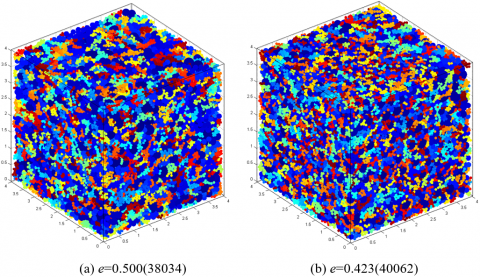
Figure 8. 3D graphics of the first group of particle sets
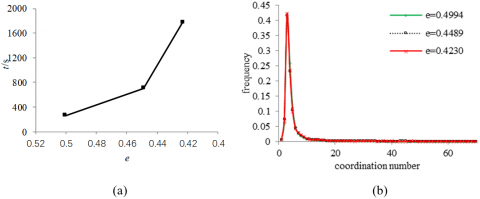
Figure 9. The first group of results sketches (number of particles 38000-40000)
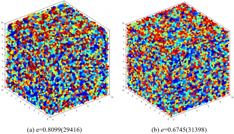
Figure 10. 3D graphics of the second group of particle sets
Figure 11. The second group of results (number of particles 27400-29500)
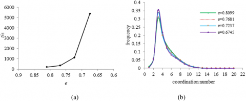
The density of stacking sets in the first group ranged from 0.667 to 0.703 (pore ratio e: 0.422 to 0.499), far exceeding the density 0.558 of reference [24]. The density of stacking sets in the second group (as shown in Figure 10 and Figure 11) ranged from 0.553 to 0.597, covering 0.575 of reference [24].
Similarly, as the difference in particle radius becomes smaller, to reach a larger particle density be more difficult, and the maximum coordination number of particles decreases from 70 to 20. With the decrease of pore ratio, the time of particle formation increases rapidly.
3.3 Generation rate
The result of the particle formation rate is shown in Figure 12. The relationship between the time when the particle set is generated and the number of particles is shown in Figure 13.
Figure 12. Velocity-time curve of particle number generation
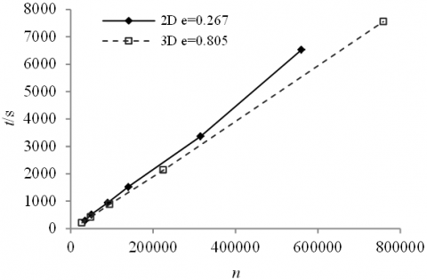
Figure 13. The relation between the time of generating particle sets and the number of particles
As can be seen from the particle formation rate (Figure 12), the granule set of lager void ratio generated faster and the target number is reached faster. The generation rate curve can be roughly divided into two stages. The first is the rapid particle generation stage. In this stage, the particles are still relatively sparse, with a high success rate and a high rate of particle generation. The second stage is the fine particles continuous fill the gaps between coarse particles, with the increase of particle density, gaps between particles decreases and granular successful probability is reduced. When certain conditions are met, the Reshape function works, constantly adjust the position between the particles to allow more particles to fill in.
To compare the relationship between the number of particles generated and the time, choose the same particle size distribution (Table 1 and Table 2) to generate the accumulation body according to the specified pore ratio, and test the relationship between the number of particles generated and the time. As can be seen from Figure 13, 2D and 3D showed a good linear relationship, 2D generated 560000 particles took nearly 1.8h, 3D generated 760000 particles took nearly 2.1h, it is ideal in the generation speed. Meanwhile, the results in Figure 13 shows that, under some conditions, the rate of 3D generation is slightly faster than that of 2D generation, which is mainly due to the fact that there is an extra degree of freedom in space in the generation process of 3D space, which leads to a higher probability of successful particle generation in space, resulting in a shorter time.
3.4 Comparison with other methods
The comparison results of generating particle sets using different methods are shown in Table 3.
Table 3. Comparisons of particle sets generated by different methods
|
2D |
The first group |
The second group |
||||
|
The proposed method |
Document [25] |
Document [23] |
The proposed method |
Document [25] |
Document [23] |
|
|
Particle number |
24901 |
37977 |
1102 |
35003 |
49533 |
38953 |
|
Particle density |
0.789 |
0.816 |
0.801 |
0.826 |
0.816 |
0.826 |
|
Time/s |
290 |
116.2 |
0.801 |
51.9 |
244.6 |
36.36 |
|
3D |
The first group |
The second group |
||||
|
The proposed method |
Document [8] |
Document [24] |
The proposed method |
Document [26] |
Document [24] |
|
|
Particle number |
38034 |
26787 |
28770 |
29416 |
33738 |
40981 |
|
Particle density |
0.667 |
0.529 |
0.575 |
0.553 |
0.494 |
0.592 |
|
Time /s |
262 |
181 |
97 |
210 |
1.01 |
179.69 |
Current most geometry or geometric and physical methods generation algorithm has a significant flaw, not under specified graded according to the need for specified void ratio (density) of particles, and it can only be fixed algorithm based on randomly generated intensity is fixed set of particles, and other auxiliary methods through implementation, such as grading. According to the natural accumulation law of particles, this paper adopts the mode of filling coarse particles first and then fine particles and adjusts the current position of particles under certain conditions to provide more space for newly generated particles, to achieve a higher density. Simulation results show that the larger the difference in particle radius, the easier it is to generate a set of particles with high density, which requires less time, and the larger the maximum coordination number of particles. Under the specified particle gradation, the method proposed in this paper can generate particle sets with higher density, but it takes a little more time than other methods. However, the required density can be adjusted according to the simulation needs.
Supported by the National Natural Science Foundation of China (NO. 41602295).
[1] Webb, M.D., Davis, I.L. (2006). Random particle packing with large particle size variations using reduced-dimension algorithms. Powder Technology, 167(1): 10-19. http://doi.org/ 10.1016/j.powtec.2006.06.003
[2] Jiang, S.Q., Ye, Y.X., Tan, Y.Q., Liu, S.S., Liu, J.G., Zhang, H., Yang, D.M. (2018). Discrete element simulation of particle motion in ball mills based on similarity. Powder Technology, 335: 91-102. http://doi.org/10.1016/j.powtec.2018.05.012
[3] Munjiza, A., Rougier, E., Knight, E.E., Zhou, L. (2018). Discrete element and particle methods. In: Altenbach H., Öchsner A. (eds) encyclopedia of continuum mechanics. Springer, Berlin, Heidelberg. https://doi.org/10.1007/978-3-662-53605-6 16-1
[4] Zhou, L., Rougier, E., Knight, E.E., Frash, L., Carey, J.W., Viswanathan, H. (2016). A non-locking composite tetrahedron element for the combined finite discrete element method. Engineering Computations, 33(7): 1929-1956. https://doi.org/10.1108/EC-09-2015-0268
[5] Keppler, I., Hudoba, Z., Oldal, I., Csatar, A., Fenyvesi, L. (2015). Discrete element modeling of vibrating tillage tools. Engineering Computations, 32(2): 308-328. https://doi.org/10.1108/ec-10-2013-0257
[6] Bagi, K. (2005). An algorithm to generate random dense arrangements for discrete element simulations of granular assemblies. Granular Matter, 7(1): 31-43. https://doi.org/ 10.1007/s10035-004-0187-5
[7] Gensane, T., Ryckelynck, P. (2008). Producing dense packings of cubes. Discrete Mathematics, 308(22): 5230-5245. https://doi.org/10.1016/j.disc.2007.09.047
[8] Han, K., Feng, Y.T., Owen, D.R.J. (2005). Sphere packing with a geometric based compression algorithm. Powder Technology, 155(1): 33-41. https://doi.org/10.1016/j.powtec.2005.04.055
[9] Bagi, K. (1993). A quasi-static numerical model for micro-level analysis of granular assemblies. Mechanics of Materials, 16(1): 101-110. https://doi.org/10.1016/0167-6636(93)90032-M
[10] Esnault, V.P.B., Roux, J.N. (2013). 3D numerical simulation study of quasistatic grinding process on a model granular material. Mechanics of Materials, 66: 88-109. https://doi.org/10.1016/j.mechmat.2013.07.018
[11] Esnault, V.P.B., Roux, J.N. (2013). Numerical simulation study of quasistatic grinding process on a model granular material. Mechanics of Materials, 66(1): 88-109. https://doi.org/10.1016/j.mechmat.2013.07.018
[12] Zheng, H., Zhang, P., Du, X.L. (2016). Dual form of discontinuous deformation analysis. Computer Methods in Applied Mechanics and Engineering, 305: 196-216. https://doi.org/ 10.1016/j.cma.2016.03.008
[13] Beyabanaki, S.A.R., Bagtzoglou, A. (2012). Three-dimensional discontinuous deformation analysis (3-d dda) method for particulate media applications. Geomechanics & Geoengineering, 7(4): 15-15. https://doi.org/10.1080/17486025.2012.714477
[14] Benabbou, A., Borouchaki, H., Laug, P., Lu, J. (2010). Numerical modeling of nanostructured materials. Finite Elements in Analysis & Design, 46(1): 165-180. https://doi.org/ 10.1016/j.finel.2009.06.030
[15] Ng, T.T., Lin, X. (1997). A three dimensional discrete element model using arrays of ellipsoids. Géotechnique, 47(2): 319-329. https://doi.org/10.1680/geot.1997.47.2.319
[16] Mazzucco, G., Pomaro, B., Salomoni, V.A., Majorana, C.E. (2018). Numerical modelling of ellipsoidal inclusions. Construction & Building Materials, 167: 317-324. https://doi.org/10.1016/j.conbuildmat.2018.01.160
[17] Zhou, Z.Y., Zou, R.P., Pinson, D., Yu, A. (2011). Dynamic simulation of the packing of ellipsoidal particles. Industrial & Engineering Chemistry Research, 50(16): 287-291. https://doi.org/10.1021/ie200862n
[18] Feng, Y.T., Han, K., Owen, D.R.J. (2003). Filling domains with disks: an advancing front approach. International Journal for Numerical Methods in Engineering, 56(5): 699-713. https://doi.org/10.1002/nme.583
[19] Seblany, F., Homberg, U., Vincens, E., Winkler, P., Witt, K.J. (2018). Merging criteria for defining pores and constrictions in numerical packing of spheres. Granular Matter, 20(3): 37-37. https://doi.org/10.1007/s10035-018-0808-z
[20] Morfa, C.A.R., Morales, I.P.P., Farias, M.M.D., Navarra, E.O.I.D., Valera, R.R., Casañas, H.D.G. (2016). General advancing front packing algorithm for the discrete element method. Computational Particle Mechanics, 5(1): 1-21. https://doi.org/10.1007/s40571-016-0144-1
[21] Munjiza, A., Andrews, K.R.F. (1998). Nbs contact detection algorithm for bodies of similar size. International Journal for Numerical Methods in Engineering, 43(1): 131-149. https://doi.org/10.1002/(SICI)1097-0207(19980915)43:13.0.CO;2-S
[22] Podlozhnyuk, A., Pirker, S., Kloss, C. (2017). Efficient implementation of superquadric particles in discrete element method within an open-source framework. Computational Particle Mechanics, 4(1): 101-118. https://doi.org/10.1007/s40571-016-0131-6
[23] Fang, X.W., Liu, Z.Y., Tan, J.R. (2011). Algorithm with hybrid method based for sphere packing in two-dimensional region. Journal of Zhejiang University (Engineering Science), 45(4): 650-655. https://doi.org/10.3785/j.issn.1008-973X.2011.04.010
[24] Fang, X., Liu, Z., Tan, J. (2011). An algorithm for particle packing in 3d space by considering geometric and physical factors. Jisuanji Fuzhu Sheji Yu Tuxingxue Xuebao/Journal of Computer-Aided Design and Computer Graphics, 23(7): 1254-1262. https://doi.org/10.1090/S0002-9939-2011-10775-5
[25] Bagi, K. (2005). An algorithm to generate random dense arrangements for discrete element simulations of granular assemblies. Granular Matter, 7(1): 31-43. https://doi.org/10.1007/s10035-004-0187-5
[26] Benabbou, A., Borouchaki, H., Laug, P., Lu, J. (2010). Geometrical modeling of granular structures in two and three dimensions. application to nanostructures. International Journal for Numerical Methods in Engineering, 80(4): 425-454. https://doi.org/10.1002/nme.2644