Van Quang Vu![]() | Gia Thinh Bui*
| Gia Thinh Bui*![]() | Huu Vinh Dang
| Huu Vinh Dang![]() | Anh Tuan Dinh
| Anh Tuan Dinh![]()
© 2024 The authors. This article is published by IIETA and is licensed under the CC BY 4.0 license (http://creativecommons.org/licenses/by/4.0/).
OPEN ACCESS
Underwater vehicles are now mainly researched using the 6-DOF equations of motion. The research on 4-DOF Autonomous Underwater Vehicles (AUV) for small Underwater Vehicles regularly focuses on fully actuated control algorithms. Research on underactuated systems has been conducted frequently for surface ships, while 4-DOF underactuated AUV using a nonlinear control system has received little attention. Little research focuses on devices with quadrotor UAV configuration, also known as QUV, but evaluations have yet to be conducted to advise on which controller to use for different cases. Therefore, in this article, the authors focus on building a control algorithm for an AUV object that lacks a typical recursive executive structure, which is the Backstepping controller when dividing the 4-order strict backpropagation nonlinear system into subsystems to design feedback controllers and Lyapunov control functions for each subsystem. Using this same approach, the authors built a controller that combines Backstepping controller and Hierarchical Sliding Mode Controller (HSMC). This is the guiding premise for research on improving the quality of 4-DOF AUV control before comparing and evaluating the two controllers for specific cases. Newly proposed algorithms and stability analyses are based on Lyapunov's theory, and an evaluation survey is carried out through simulation by Matlab software.
Autonomous Underwater Vehicle, Backstepping controller, Hierarchical Sliding Mode Controller, underactuated
An underactuated system is a control system with fewer actuators than the number of degrees of freedom or model variables, which means several output variables of the system depend on the same input variable [1]. In recent years, the underactuated system has been increasingly researched [2, 3]. Systems such as ships, submarines, aircraft, spacecraft, and robots are designed with underactuated systems to reduce costs or weight and energy consumption [4, 5]. In some cases, the system becomes underactuated due to defective actuators. When reducing the number of actuators, developing control techniques is more necessary and complex than the fully actuated systems [6, 7].
AUV (Autonomous et al.) operates underwater and is affected by unknown factors such as depth, pressure, and ocean currents [8, 9], which are not calculated accurately; even the kinetic properties of AUV are constant over time, such as material loss, ship weight, change in ship center of gravity [10, 11]. Improving the quality of trajectory tracking control of AUVs requires the use of modern nonlinear control theory [12, 13].
Depending on each type of AUV, different controllers will be used. Each controller will have its advantages and disadvantages. For example, in the backstepping technique, the control law of the rear system depends on the derivative of the control law of the front subsystem, which causes operand explosion in the Backstepping technique, especially when the system is multilevel [14]. HSMC control is a good solution for nonlinear systems [15, 16]. Nevertheless, it has the potential to induce high-frequency oscillations, impacting the actuators, dissipating energy, and generating wing oscillations in the AUV, consequently resulting in instability [17, 18]. Therefore, the evaluation to obtain solutions for specific cases is necessary. With such details, the rest of the Article is outlined as follows. The AUV model with 4 degrees of freedom is introduced in section 2. Section 3 presents the indirect control method for Backstepping an underactuated system and the direct control method for an underactuated AUV. Comparison and control quality assessment between the two methods are presented in section 4 on Matlab simulink before concluding section 5.
The kinematic model of AUV is based on mechanical theory, kinetics principles, and statics fundamentals. This model serves as the foundation for designing control systems tailored to achieve specific objectives for the vehicle. Generally, the motion of an AUV can be characterized by the 4-degree-of-freedom (DOF) equation of motion, encompassing key components such as direction of motion, forces and moments, velocity, and position, as outlined in Table 1. This includes motion along the x-axis (surge), y-axis (sway), z-axis (heave), and rotation about the z-axis (yaw).
Table 1. Parameters in the 4-DOF AUV model
|
DOF |
Target |
Force and Moments |
Velocities |
Positions and Angles |
|
1 |
Motion in x direction (surge) |
X |
u |
x |
|
2 |
Motion in y direction (sway) |
Y |
v |
y |
|
3 |
Motion in z direction (heave) |
Z |
w |
z |
|
4 |
Rotation about z axis (yaw) |
N |
r |
ψ |
The AUV 4 DOF motion model includes: η=[x,y,z,ψ]T is the position vector of the ship along the axes of Ox, Oy, Oz and the ship's navigation angle around the axis of Oz; v=[u,v,w,r]T is the long velocity vector in the directions of Ox, Oy, Oz and the rotational speed around the Oz axis.
According to Eq. (1), we rewrite the kinematic equation of AUV as follows:
$\left\{\begin{array}{l}\dot{\eta}=J(\eta) v \\ M \dot{v}+C(v) v+D(v) v=\tau\end{array}\right.$ (1)
τ=[X,Y,Z,N]T is the control force and torque vector in the Oxyz dynamic coordinate system.
M is the systematic inertia matrix of AUV, C(v) is the Coriolis matrix and the centripetal force of AUV.
The rotation matrix on the Oz axis is shown as follows:
$J(\eta)=\left[\begin{array}{llll}\cos (\psi) & -\sin (\psi) & 0 & 0 \\ \sin (\psi) & \cos (\psi) & 0 & 0 \\ 0 & 0 & 1 & 0 \\ 0 & 0 & 0 & 1\end{array}\right]=\left[\begin{array}{ll}J_{11} & J_{12} \\ J_{21} & J_{22}\end{array}\right]$ (2)
Systemic inertia matrix is shown as follows:
$\begin{aligned} & M=\left[\begin{array}{llll}m+X_{\dot{u}} & 0 & X_{\dot{\mathrm{w}}} & -m y_g \\ 0 & m+Y_{\dot{v}} & 0 & Y_{\dot{r}}+m x_g \\ Z_{\dot{u}} & 0 & m+Z_{\dot{\mathrm{w}}} & 0 \\ -m y_g & m x_g+N_{\dot{v}} & 0 & I_z+N_{\dot{r}}\end{array}\right] =\left[\begin{array}{ll}M_{11} & M_{12} \\ M_{21} & M_{22}\end{array}\right] \\ & \end{aligned}$ (3)
Coriolis matrix and systemic centripetal force are shown as follows:
$\begin{aligned} C= & {\left[\begin{array}{llll}0 & -m r & 0 & -m x_g r-a_2 \\ m r & 0 & 0 & -m y_g r+a_1 \\ 0 & 0 & 0 & 0 \\ m x_g r+a_2 & m y_g r-a_1 & 0 & 0\end{array}\right] }=\left[\begin{array}{ll}C_{11} & C_{12} \\ C_{21} & C_{22}\end{array}\right]\end{aligned}$ (4)
Hydrodynamic attenuation matrix is shown as follows:
$\begin{aligned} & D(v) \\ & =\left[\begin{array}{llll}X_u+X_{u|u|}|u| & 0 & 0 & 0 \\ 0 & Y_v+Y_{v|v|}|v| & 0 & 0 \\ Z_0|u| & 0 & Z_w+Z_{w|w|}|w| & 0 \\ 0 & 0 & 0 & K_p+K_{p|p|}|p|\end{array}\right] =\left[\begin{array}{ll}D_{11} & D_{12} \\ D_{21} & D_{22}\end{array}\right]\end{aligned}$ (5)
with matrices of $M, J(\eta), C(v), D(v)$ to satisfy the following properties: $M=M^T>0 ; C(v)=C^T(v) ; D(v)>0$ and $J(\eta)$ is the matrix rotating about the Oz axis and is the orthogonal matrix $J^{-1}(\eta)=J^T(\eta)$.
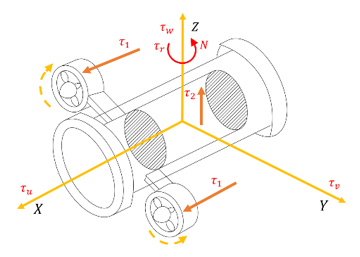
The four-degree-of-freedom motion model of AUV includes: $\eta=[x, y, z, \psi]^T$ is the position vector of the ship along $\eta=[x, y, z, \psi]^T$ axes and the angle that directs the ship to rotate around the $O z$ axis; $v=[u, v, \mathrm{w}, r]^T$ is the long velocity vector in the $O x, O y, O z$ directions and the speed of rotation around the $O z$ axis. According to Eq. (1), $\tau$ – which is the force and torque produced by the performance mechanism of the AUV, these forces and torque are performed by $\tau=\left[\tau_u, \tau_v, \tau_w, \tau_r\right]^T$, in which: $\tau_u-$ – the force that causes the AUV to slide vertically along the X-axis direction, $\tau_v–$ the force that causes the AUV to slide horizontally in the Y-axis direction, $\tau_w-$ the force that causes AUV to slide horizontally in the Z-axis direction, $\tau_r-$ the torque that rotates around the z-axis causes a change in AUV’s direction.
According to Fossen and Paulsen [19], the four-degree-of-freedom AUV model is considered on the horizontal plane with a mathematical model such as Eq. (1). If the force component t has all four components $\tau=\left[\tau_u, \tau_v, \tau_w, \tau_r\right]^T$ and $v=[u, v, \mathrm{w}, r]^T$ then the mathematical model on the horizontal plane is called the fully actuated ship model. On the other hand, if $\tau_v, \tau_r=0$, in the mathematical model of AUV, if there is no force component that causes horizontal sliding and turning (the element does not have a horizontal thrust mechanism and a rudder) towards the y-axis, the computational model on the horizontal plane is called the Underactuated model.
This is a typical mathematical model for the AUV with only two performing mechanisms, a rear thruster and vertical axis engine, such as the operating model of Quadrotor UAV, also known as QUV, as shown in Figure 1.
Figure 1. Analysis of underactuated 4-DOF AUV force
An AUV is considered an underactuated device when the number of input control signals is less than the number of control state variables (or degrees of freedom) [2]. NCS separates the mathematical model Eq. (1) into two parts: the underactuated system and the fully actuated system. The position vector $\eta=\left[\begin{array}{ll}\eta_1 & \eta_2\end{array}\right]^T$ will be divided into two parts: $\eta_1=\left[\begin{array}{ll}x & z\end{array}\right]^T$ for underactuated system and $\eta_2=\left[\begin{array}{ll}y & \psi\end{array}\right]^T$ for fully actuated system. Similarly, the velocity vector $v$ is also divided into two parts with $v=\left[\begin{array}{ll}v_1 & v_2\end{array}\right]^T$. The AUV dynamic Eq. (1) is rewritten as follows:
$\left\{\begin{array}{l}\dot{\eta}_1=J_{11} v_1+J_{12} v_2 \\ \dot{\eta}_2=J_{21} v_1+J_{22} v_2 \\ M_{11} \dot{v}_1+\left(C_{11}+D_{11}\right) v_1+M_{12} \dot{v}_2+\left(C_{12}+D_{12}\right) v_2=\tau \\ M_{21} \dot{v}_1+\left(C_{21}+D_{21}\right) v_1+M_{22} \dot{v}_2+\left(C_{22}+D_{22}\right) v_2=0\end{array}\right.$ (6)
Since $M_{22}$ is a positive definite matrix, from the fourth equation in Eq. (6), it follows that:
$\begin{gathered}\dot{v}_2=-M^{-1}{ }_{22}\left[M_{21} \dot{v}_1+\left(C_{21}+D_{21}\right) v_1+\left(C_{22}\right.\right. \left.\left.+D_{22}\right) v_2\right]\end{gathered}$ (7)
Substituting Eq. (7) into the third equation in Eq. (6):
$\begin{aligned} & M_{11} \dot{v}_1+\left(C_{11}+D_{11}\right) v_1 \\ & -M_{12} M^{-1}{ }_{22}\left[M_{21} \dot{v}_1+\left(C_{21}\right.\right. \\ & \left.\left.+D_{21}\right) v_1+\left(C_{22}+D_{22}\right) v_2\right] \\ & +\left(C_{12}+D_{12}\right) v_2=\tau \\ & \Leftrightarrow\left(M_{11}-M_{12} M^{-1}{ }_{22} M_{21}\right) \dot{v}_1 \\ & +\left(\left(C_{11}+D_{11}\right)-M_{12} M^{-1}{ }_{22}\left(C_{21}\right.\right. \\ & \left.\left.+D_{21}\right)\right) v_1 \\ & +\left(\left(C_{12}+D_{12}\right)-M_{12} M^{-1}{ }_{22}\left(C_{22}\right.\right. \\ & \left.\left.+D_{22}\right)\right) v_2=\tau \\ & \end{aligned}$
Simplify equation, the following is calculated:
$\bar{M} \dot{v}_1+\bar{C}_1 v_1+\bar{C}_2 v_2=\tau$ (8)
$\begin{aligned} \bar{M} & =M_{11}-M_{12} M^{-1}{ }_{22} M_{21} \\ \text { with: } \bar{C}_1 & =\left(C_{11}+D_{11}\right)-M_{12} M^{-1}{ }_{22}\left(C_{21}+D_{21}\right) \\ \bar{C}_2 & =\left(C_{12}+D_{12}\right)-M_{12} M^{-1}{ }_{22}\left(C_{22}+D_{22}\right)\end{aligned}$
Since $\bar{M}-$ the invertible matrix is positive definite, from Eq. (8), it follows that:
$\dot{v}_1=\bar{M}^{-1}\left(-\bar{C}_1 v_1-\bar{C}_2 v_2\right)+\bar{M}^{-1} \tau$ (9)
Substituting Eq. (8) into Eq. (6):
$\begin{gathered}\Leftrightarrow \dot{v}_2=-M^{-1}{ }_{22}\left[M_{21} \bar{M}^{-1}\left(-\bar{C}_1 v_1-\bar{C}_2 v_2\right)+\right. \\ \left.\left(C_{21}+D_{21}\right) v_1+\left(C_{22}+D_{22}\right) v_2\right]-M^{-1}{ }_{22} M_{21} \bar{M}^{-1} \tau\end{gathered}$
Replacing Eq. (8) and Eq. (9) into the system of Eq. (6), it follows that the system of dynamic equations of AUV is calculated as follows:
$\left\{\begin{array}{l}\eta_1=J_{11} v_1 \\ \dot{v}_1=\bar{M}^{-1}\left(-\bar{C}_1 v_1-\bar{C}_2 v_2\right)+\bar{M}^{-1} \tau \\ \eta_2=J_{22} v_2 \\ v_2=-M^{-1}{ }_{22}\left[\begin{array}{c}M_{21} \bar{M}^{-1}\left(-\bar{C}_1 v_1-\bar{C}_2 v_2\right) \\ +\left(C_{21}+D_{21}\right) v_1 \\ +\left(C_{22}+D_{22}\right) v_2\end{array}\right]-M^{-1}{ }_{22} M_{21} \bar{M}^{-1} \tau\end{array}\right.$ (10)
with: $J_{12}(v)=\left[\begin{array}{ll}0 & 0 \\ 0 & 0\end{array}\right]$ and $J_{21}(v)=\left[\begin{array}{ll}0 & 0 \\ 0 & 0\end{array}\right]$
This is the system of kinematic equations after being transformed by the mechanical actuator method. The system of equations is essential for control algorithms that can be applied later. It is possible to apply in the simulation; we must build a model of the object first.
3.1 Recursion based control 4-DOF AUV controller design
The Eq. (10) is rewritten in the generalized form as follows:
$\left\{\begin{array}{l}\dot{\eta}_1=J_{11} v_1 \\ \dot{v}_1=f_1(\boldsymbol{X})+g_1(\boldsymbol{X}) \tau_1 \\ \dot{\eta}_2=J_{22} v_2 \\ \dot{v}_2=f_2(\boldsymbol{X})+g_2(\boldsymbol{X}) \tau_2\end{array}\right.$ (11)
where:
$\begin{aligned} & X=\left[\begin{array}{llll}\eta_1 & v_1 & \eta_2 & v_2\end{array}\right]^T \\ & f_1(X)=\bar{M}^{-1}\left(-\bar{C}_1 v_1-\bar{C}_2 v_2\right) \\ & g_1(X)=\bar{M}^{-1} \\ & f_2(X)=-M^{-1}{ }_{22}\left[\begin{array}{c}M_{21} \bar{M}^{-1}\left(-\bar{C}_1 v_1-\bar{C}_2 v_2\right) \\ +\left(C_{21}+D_{21}\right) v_1 \\ +\left(C_{22}+D_{22}\right) v_2\end{array}\right] \\ & g_2(X)=-M^{-1}{ }_{22} M_{21} \bar{M}^{-1} \\ & \end{aligned}$
The definition of the error vector between the output signal and the set signal is as follows:
$e(t)=\left[\begin{array}{l}e_1 \\ e_3\end{array}\right]=\left[\begin{array}{l}\eta_1-\eta_{1 d} \\ \eta_2-\eta_{2 d}\end{array}\right]$ (12)
Consider the Eq. (11) as two subsystems of Eq. (13), Eq. (14) with control signals $\tau_1, \tau_2$ for each system
$\left\{\begin{array}{l}\dot{\eta}_1=J_{11} v_1 \\ \dot{v}_1=f_1(\boldsymbol{X})+g_1(\boldsymbol{X}) \tau_1\end{array}\right.$ (13)
$\left\{\begin{array}{l}\dot{\eta}_2=J_{22} v_2 \\ \dot{v}_2=f_2(\boldsymbol{X})+g_2(\boldsymbol{X}) \tau_2\end{array}\right.$ (14)
The system control signal of Eq. (12) is selected according to the following law:
$\tau=\alpha \tau_1+\beta \tau_2$ (15)
with $\alpha, \beta$ as positive constants.
Eq. (13) and Eq. (14) are secondary tight backpropagation, according to the Backstepping technique, to determine the control signal $\tau_1, \tau_2$:
$\tau_1=g_1^{-1}(\boldsymbol{X})\left(-c_2 e_2-J_{11}^T e_1-f_1(\boldsymbol{X})+\dot{\alpha}_1\right)$ (16)
with $c_2$ as a positive constant
$\tau_2=g_2^{-1}(\boldsymbol{X})\left(-c_4 e_4-J_{22}^T e_3-f_2(\boldsymbol{X})+\dot{\alpha}_2\right)$ (17)
with $e_3=\eta_2-\eta_{2 d} e_4=\dot{\eta}_2-\dot{\eta}_{2 d}, \alpha_2=J_{22}^{-1}\left(-c_3 e_3+\dot{\eta}_{2 d}\right)$, $c_3, c_4$ as positive constants.
Substitute $\tau_1, \tau_2$ into the Eq. (15) to calculate:
$\begin{aligned} & \tau=\alpha \cdot g_1^{-1}(\boldsymbol{X})\left(-c_2 e_2-J_{11}^T e_1-f_1(\boldsymbol{X})+\dot{\alpha}_1\right)+\beta \cdot g_2^{-1}(\boldsymbol{X})\left(-c_4 e_4-J_{22}^T e_3\right.\left.-f_2(\boldsymbol{X})+\dot{\alpha}_2\right)\end{aligned}$ (18)
3.2 Separation sliding manifold based 4-DOF AUV controller design
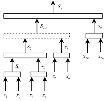
The theory of a separation sliding manifold based on a 4-DOF AUV controller design has been fully presented in the document [20] for the class of MIMO systems lacking actuators. In essence, a Separation sliding manifold is a combination of a Backstepping technique with sliding control. The HSMC structure is presented in Figure 2.
Figure 2. Structure of the HSMC
The HSMC control method is shown as follows:
$\left\{\begin{array}{c}\dot{x}_1=x_2 \\ \dot{x}_2=f_1(X)+g_1(X) \tau \\ \dot{x}_3=x_4 \\ \dot{x}_4=f_2(X)+g_2(X) \tau \\ \vdots \\ \dot{x}_{2 n-1}=x_{2 n} \\ \dot{x}_{2 n}=f_n(X)+g_n(X) \tau\end{array}\right.$ (19)
where, $X=\left[\begin{array}{llll}x_1 & x_2 & \ldots & x_{2 n}\end{array}\right]^T$ is the state variable vector; $f_i$ is a bounded nonlinear function; $g_i$ is larger than zero and has an equilibrium point at the origin.
From the system of equations (11), we rewrite it in a generalized form as follows:
$\left\{\begin{aligned} & \dot{\eta}_1=J_{11} v_1 \\ \dot{v}_1= & f_1(X)+g_1(X) \tau \\ & \dot{\eta}_2=J_{22} v_2 \\ \dot{v}_2= & f_2(X)+g_2(X) \tau\end{aligned}\right.$ (20)
where,
$X=\left[\begin{array}{llll}\eta_1 & v_1 & \eta_2 & v_2\end{array}\right]^T$
$\begin{gathered}f_1(X)=\bar{M}^{-1}\left(-\bar{C}_1 v_1-\bar{C}_2 v_2\right) \\ g_1(X)=\bar{M}^{-1} \\ f_2(X)=-M^{-1}{ }_{22}\left[M_{21} \bar{M}^{-1}\left(-\bar{C}_1 v_1-\bar{C}_2 v_2\right)+\left(C_{21}+D_{21}\right) v_1\right. \\ \left.+\left(C_{22}+D_{22}\right) v_2\right] \\ g_2(X)=-M^{-1}{ }_{22} M_{21} \bar{M}^{-1}\end{gathered}$
The definition of errors between the system reponses and the desired references are:
$e(t)=\left[\begin{array}{l}e_1 \\ e_2 \\ e_3 \\ e_4\end{array}\right]=\left[\begin{array}{l}\eta_1-\eta_{1 d} \\ v_1 \\ \eta_2-\eta_{2 d} \\ v_2\end{array}\right]$ (21)
In this case, $\eta_{1 d}$ is the desired postion vetor of the device in axes $O x, O y$; $\eta_{2 d}$ is the vector of desired postion in the $O z$ axes and navigation angle of AUV.
The sliding surface is summarized by:
$\left\{\begin{array}{l}s_1=k_1 e_1+e_2 \\ s_2=k_2 e_3+e_4 \\ s=\lambda s_1+\beta s_2\end{array}\right.$ (22)
where, $k_1, k_2$ are positive constants; $\lambda, \beta$ are positive parameters.
According to HSMC method, the controller signal is fomulated by:
$\tau=\tau_{e q}+\tau_{s \mathrm{~W}}$ (23)
with $\tau_{e q}$ is the equivalent control that is used to control subsystem in controller structure of HSMC, $\tau_{s w}$ is switch control for the following sliding surface system.
In order to ensure the stability of SAUV system, a Lyapunov function is considered by:
$V=\frac{1}{2} S^T S$ (24)
For futher analysis, let us derivative of the sliding surface as follows:
$\begin{aligned} & \frac{d V}{d t}=S^T \cdot \dot{S} \\ & =S^T \cdot\left[\lambda \dot{s}_1+\beta \dot{s}_2\right] \\ & =S^T \cdot\left[\begin{array}{c}\lambda\left(k_1 J_{11} v_1+f_1+g_1 \tau-k_1 \dot{\eta}_{1 d}\right) \\ +\beta\left(k_2 J_{22} v_2+f_2+g_2 \tau-k_2 \dot{\eta}_{2 d}\right)\end{array}\right] \\ & =s^T \cdot\left[\begin{array}{c}\lambda\left(\begin{array}{c}k_1 J_{11} v_1+f_1+g_1\left(\tau_{e q 1}+\tau_{s \mathrm{w} 1}\right. \\ \left.+\tau_{e q 2}+\tau_{s \mathrm{w} 2}\right)-k_1 \dot{\eta}_{1 d}\end{array}\right) \\ +\beta\left(\begin{array}{c}k_2 J_{22} v_2+f_2+g_2\left(\tau_{e q 1}+\tau_{s \mathrm{w} 1}\right. \\ \left.+\tau_{e q 2}+\tau_{s \mathrm{w} 2}\right)-k_2 \dot{\eta}_{2 d}\end{array}\right)\end{array}\right] \\ & =S^T \cdot\left[\begin{array}{c}\lambda\left(k_1 J_{11} v_1+f_1+g_1 \tau_{e q 1}-k_1 \dot{\eta}_{1 d}\right) \\ +\beta\left(k_2 J_{22} v_2+f_2+g_2 \tau_{e q 2}-k_2 \dot{\eta}_{2 d}\right) \\ +\tau_{s \mathrm{w} 1}\left(\lambda g_1+\beta g_2\right)+\tau_{s \mathrm{w} 2}\left(\lambda g_1+\beta g_2\right) \\ +\lambda g_1 \tau_{e q 2}+\beta g_2 \tau_{e q 1}+k . S+\sigma \operatorname{sgn}(S) \\ -(k . S+\sigma \operatorname{sgn}(S))\end{array}\right] \\ & \end{aligned}$ (25)
where, $k$ is the parameter that can be used to eliminate the chattering phenomena; $u_{e q}=u_{e q 1}+u_{e q 2}$, $u_{s \mathrm{w}}=u_{s \mathrm{w} 1}+u_{s \mathrm{w} 2}$. Moreover, the stability of the SAUV system is guaranteed if
$\left\{\begin{array}{l}\tau_{e q 1}=-g_1^{-1} \cdot\left(k_1 J_{11} v_1+f_1-k_1 \dot{\eta}_{1 d}\right) \\ \tau_{e q 2}=-g_2^{-1} \cdot\left(k_2 J_{22} v_2+f_2-k_2 \dot{\eta}_{2 d}\right) \\ \tau_{s w 2}=-\tau_{s w 1}-\left(\begin{array}{c}\lambda g_1 \\ +\beta g_2\end{array}\right)^{-1}\left(\begin{array}{c}\lambda g_1 \tau_{e q 2} \\ +\beta g_2 \tau_{e q 1} \\ +k \cdot S \\ +\delta \operatorname{sgn}(S)\end{array}\right)\end{array}\right.$ (26)
which leads to
$\frac{d V}{d t}=S^T \cdot \dot{S}=-\left(k \cdot S^T S+\delta S^T \operatorname{sgn}(S)\right) \leq 0$ (27)
Thus, the control signal for HSMC scheme is aggregated as:
$\begin{gathered}\tau=\tau_{e q 1}+\tau_{s \mathrm{w} 1}+\tau_{e q 2}+\tau_{s w 2} =\left[\begin{array}{c}-g_1^{-1} \cdot\left(k_1 J_{11} v_1+f_1-k_1 \dot{\eta}_{1 d}\right) \\ -g_2^{-1} \cdot\left(k_2 J_{22} v_2+f_2-k_2 \dot{\eta}_{2 d}\right) \\ -\left(\lambda g_1+\beta g_2\right)^{-1}\left(\begin{array}{c}\lambda g_1 \tau_{e q 2}+\beta g_2 \tau_{e q 1} \\ +k . S+\delta \operatorname{sgn}(S)\end{array}\right)\end{array}\right]\end{gathered}$ (28)
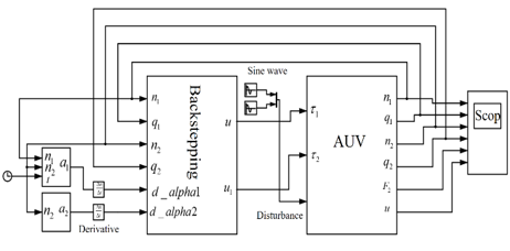
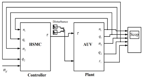
Diagram of Hierarchical sliding-mode controller (HSMC) for underactuated AUV on Matlab simulink includes input signal block, set signal, HSMC control block, and AUV operator model (with the impact of noise), output signal block (Scop) as shown in Figure 3 and Figure 4.
Figure 3. Diagram of Backstepping control simulation on Matlab simulink
Figure 4. Diagram of Hierarchical sliding-mode controller (HSMC) Simulation on Matlab simulink
To validate the effectiveness of the Backstepping controller implemented on the AUV, simulations are conducted utilizing the parameter sets outlined in Table 2, Table 3, and Table 4.
Table 2. The parameters of AUV system
|
Prameters |
Values |
Prameters |
Values |
|
$m$ |
18.5 kg |
$Z_w$ |
4.57 kg/s |
|
$x_g$ |
0.15 m |
$\dot{Z}_u$ |
0.32 kg |
|
$y_g$ |
0.15 m |
$Z_0$ |
0 |
|
$\mathrm{z}_g$ |
0 m |
$\dot{X}_{\mathrm{w}}$ |
$\begin{aligned} & -1.13 \times 10^{-6} \mathrm{~kg}\end{aligned}$ |
|
$\dot{X}_u$ |
$\begin{gathered}6.83 \times10^{-6} \mathrm{~kg} / \mathrm{s}\end{gathered}$ |
$N_r$ |
-12.32 kg.m2/rad/s |
|
$X_{u|u|}$ |
-0.58 kg/m |
$\dot{N}_v$ |
0.32 kg.m2/rad |
|
$Y_v$ |
0.08 kg/s |
$I_z$ |
1.57 kg.m2 |
|
$Y_r$ |
-1.03 kg.m/rad/s |
$N_{r|r|}$ |
$0.5 \times 10^{-3}$ kg/m |
|
$\dot{Y}_v$ |
-0.85 kg |
$N_{r|r|}$ |
$0.5 \times 10^{-6}$ |
|
$\dot{Y}_{v|v|}$ |
-0.62 kg/m |
$Z_{\mathrm{w}|\mathrm{w}|}$ |
$\begin{gathered}1.15 \times 10^{-6} \mathrm{~kg} / \mathrm{m}\end{gathered}$ |
Table 3. The parameters of Backstepping controller
|
Prameters |
Values |
Prameters |
Values |
|
$k$ |
100 |
c1 |
$c_1=\operatorname{diag}\{0.15 \quad 0.12\}$ |
|
$\delta$ |
5 |
c2 |
$c_2=\operatorname{diag}\left\{\begin{array}{ll}90 & 90\end{array}\right\}$ |
|
$k_1$ |
0.05 |
c3 |
$c_3=\operatorname{diag}\{0.2 \quad 0.2\}$ |
|
$k_2$ |
5 |
c4 |
$c_4=\operatorname{diag}\{0.1 \quad 0.1\}$ |
|
$\lambda$ |
500 |
$\eta_{1 d}$ |
Constant |
|
$\beta$ |
2.5 |
$\eta_{2 d}$ |
Constant |
Table 4. The parameters of Hierarchical Sliding Mode Controller
|
Prameters |
Values |
Prameters |
Values |
|
$k$ |
100 |
$\lambda$ |
500 |
|
$\delta$ |
5 |
$\beta$ |
2.5 |
|
$k_1$ |
0.05 |
$\eta_{1 d}$ |
$\left[\begin{array}{ll}5 & 4\end{array}\right]^T$ |
|
$k_2$ |
5 |
$\eta_{2 d}$ |
$\left[\begin{array}{ll}-4 & 0\end{array}\right]^T$ |
Declare parameters to get a characteristic line for Figure 5, Figure 6, and Figure 7 of the x-axis, the y-axis, and the z-axis with data parameters as a. timer over time and a. Data
figure(5), plot(a.time,a.Data(:,1),'blue','linewidth',3.0); hold on;
plot(a.time,x.Data,'red','linewidth',3.0); plot(a.time,a.Data(:,2),'black--','linewidth',3.0);
legend('x - Backstepping','x - HSMC, 'x - Reference');
grid on; xlabel('time [secs]');
figure(6), plot(b.time,b.Data(:,1),'blue','linewidth',3.0); hold on;
plot(b.time,y.Data,'red','linewidth',3.0);
plot(b.time,b.Data(:,2),'black--','linewidth',3.0);
legend('y - Backstepping','y - HSMC, 'y - Reference');
grid on; xlabel('time [secs]');
figure(7), plot(c.time,c.Data(:,1),'blue','linewidth',3.0); hold on;
plot(c.time,z.Data,'red','linewidth',3.0); plot(c.time,c.Data(:,2),'black--','linewidth',3.0);
legend('z - Backstepping','z - HSMC, 'z - Reference');
grid on; xlabel('time [secs]');
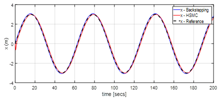
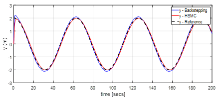
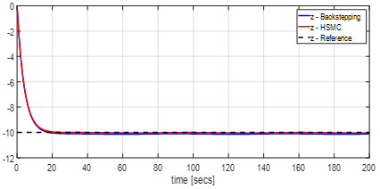
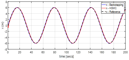
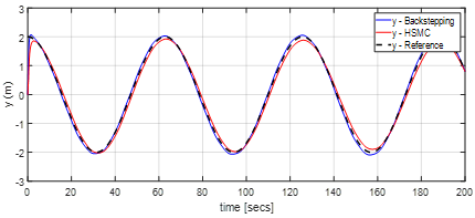
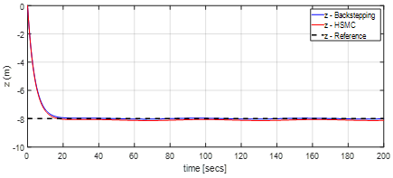
Case 1: The AUV descends to a depth of -10m below the surface water while concurrently maneuvering to the intended position with the specified values: $\eta_{1 d}=\left[\begin{array}{ll}3 \sin (0.01 t) & 2 \cos (0.01 t)\end{array}\right]^T$ and $\eta_{2 d}=\left[\begin{array}{ll}-10 & 0\end{array}\right]^T$. We intentionally influenced the system by an external disturbance on the control signal that was defined by: $\Delta=\left[\begin{array}{ll}10 \sin (0.01 t) & 5 \cos (0.01 t)\end{array}\right]^T$.
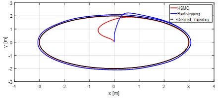
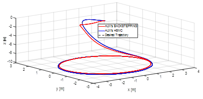
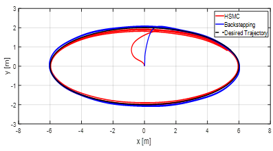
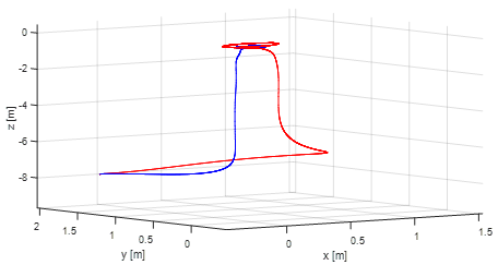
The Backstepping AUV controller grabs the x-axis position after about 18 seconds (Figure 5), the y-axis position for about 25 seconds (Figure 6), and the z-axis position for about 18 seconds (Figure 7), and the maximum overshoot is minimal in the x- and y-directions (Figure 8). Therefore, the Hierarchical Sliding Mode Controller (HSMC) responds better to trajectory tracking than the Backstepping controller under the influence of external noise. Especially with trajectory tracking on the 3D plane (Figure 9), the HSMC controller almost tracks overlapping trajectories. The article continues the comparison test in case 2 with the following parameters:
Case 2: The AUV descends to a depth of -10m below the surface water and simultaneously transitions to the desired position with the following parameters: $\eta_{1 d}=\left[\begin{array}{ll}6 \sin (0.01 t) & 2 \cos (0.01 t)\end{array}\right]^T$ and $\eta_{2 d}=\left[\begin{array}{ll}-8 & 0\end{array}\right]^T$. We intentionally influenced the system by an external disturbance on the control signal that was defined by: $\Delta=\left[\begin{array}{ll}10 \sin (0.01 t) & 5 \cos (0.01 t)\end{array}\right]^{\bar{T}}$.
Figure 5. X-axis response of AUV with 2 Backstepping controllers and HSMC in case 1
Figure 6. Y-axis response of AUV with 2 Backstepping controllers and HSMC in case 1
Figure 7. Z-axis response of AUV with 2 Backstepping controllers and HSMC in case 1
Figure 8. X-axis, Y-axis response of AUV with two controllers in case 1
Figure 9. 3D trajectory tracking AUV with two controllers
Figure 10. X-axis response of AUV with 2 Backstepping controllers and HSMC in case 2
Figure 11. Y-axis response of AUV with 2 Backstepping controllers and HSMC in case 2
Figure 12. Z-axis response of AUV with 2 Backstepping controllers and HSMC in case 2
Figure 13. X-axis, Y-axis response of AUV with two controllers in case 2
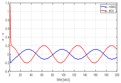
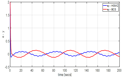
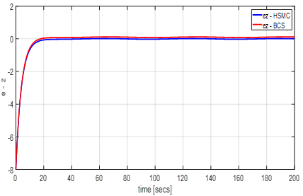
The HSMC and BCS controllers deliver good quality even when external noise is applied to the AUV. Reduce oscillation when switching around the sliding surface so that the system is more efficient when using a Hierarchical Sliding Mode Controller (HSMC) than a Backstepping Controller. The simulation values stick to the desired set value, and the overshoot is minimal. The authors specifically illustrated this result in a simulation comparing the error between the signals of the two controllers with the signal set according to the following graph. Referring to Figures 10, 11, and 12, both HSMC and BCS exhibit effective control over the AUV, demonstrating satisfactory position, velocity, and navigation angle performance. Specifically, in case 2, the system achieves tracking of position trajectories in the Ox, Oy, and Oz dimensions within 18s, 30s, and 16s, respectively. Especially with trajectory tracking on the 2D plane (Figure 13), the HSMC controller almost tracks overlapping trajectories. However, there remains an overshoot in the AUV system, as depicted in Figures 10 and 11, measuring 3.25% and 3.67%, respectively. Nevertheless, the error of the diving AUV system nearly approaches zero, with a deviation of less than 5% from the desired error band. Additionally, both weight parameters' norms converge to zero. To further assess the stability of the control performance, deliberate perturbations were introduced along the X-axis (Figure 14), Y-axis (Figure 15), Z-axis (Figure 16), and the average error relative to the set signal of both HSMC and Backstepping controllers (Figue 17).
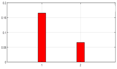
The graphs confirm the advantages of the HSMC controller, with the x-axis error being about 0.2 smaller than 0.1 (Figure 14) and the average BCS error being twice that of the HSMC (Figure 17). The asymptotic points around the origin of BCS is also twice that of HSMC (Figure 18).
Figure 14. Error compared to the X-axis set signal of the HSMC and Backstepping controllers
Figure 15. Error compared to the Y-axis set signal of the HSMC and Backstepping controllers
Figure 16. Error compared to the Z-axis set signal of the HSMC and Backstepping controllers
Figure 17. Average error compared to the set signal of the HSMC and Backstepping controllers
Figure 18. Error in 3D spaces of the HSMC and Backstepping controllers
The article successfully compared underactuated AUV controllers with each other to give an evaluation for users to choose controllers. In the case of choosing two nonlinear controllers, HSMC should be preferred because of its superior control quality, such as direct control of online data collection, slight overshoot, and shorter setup time. If users want to spend less time on design but can still guarantee quality, they should choose BCS. In the coming time, the research group will combine intelligent controllers to optimize the control algorithm further to achieve high efficiency in controlling the AUV model the research group built.
[1] Van Nguyen, T., Le, H.X., Tran, H.V., Nguyen, D.A., Nguyen, M.N., Nguyen, L. (2021). An efficient approach for simo systems using adaptive fuzzy hierarchical sliding mode control. In 2021 IEEE International Conference on Autonomous Robot Systems and Competitions (ICARSC), Santa Maria da Feira, Portugal, pp. 85-90. https://doi.org/10.1109/ICARSC52212.2021.9429793
[2] LeBlanc, G. (2011). Design and simulation of a control continuum for tetherless underwater vehicles. Faculty of Graduate Studies Online Theses, Dalhousie University.
[3] Van, T.N., Van, P.D., Cong, T.N., Chi, H.N. (2023). Modeling and designing hierarchical sliding mode controller for a 4-DOF solar autonomous underwater vehicles. International Journal of Mechanical Engineering and Robotics Research, 12(5): 275-283. https://doi.org/10.18178/ijmerr.12.5.275-283
[4] Zhang, J.L., Xiang, X.B., Zhang, Q., Li, W.J. (2020). Neural network-based adaptive trajectory tracking control of underactuated AUVs with unknown asymmetrical actuator saturation and unknown dynamics. Ocean Engineering, 218: 108193. https://doi.org/10.1016/j.oceaneng.2020.108193
[5] Eichhorn, M., Ament, C., Jacobi, M., Pfuetzenreuter, T., Karimanzira, D., Bley, K., Boer, M., Wehde, H. (2018). Modular AUV system with integrated real-time water quality analysis. Sensors, 18(6): 1837. https://doi.org/10.3390/s18061837
[6] Wu, Z.W., Peng, H.S., Hu, B., Feng, X.D. (2021). Trajectory tracking of a novel underactuated AUV via nonsingular integral terminal sliding mode control. IEEE Access, 9: 103407-103418. https://doi.org/10.1109/ACCESS.2021.3098800
[7] Le, V.A., Le, H.X., Nguyen, L., Phan, M.X. (2019). An efficient adaptive hierarchical sliding mode control strategy using neural networks for 3D overhead cranes. International Journal of Automation and Computing, 16(5): 614-627. https://doi.org/10.1007/s11633-019-1174-y
[8] Patil, P.V., Khan, M.K., Korulla, M., Nagarajan, V., Sha, O.P. (2022). Design optimization of an AUV for performing depth control maneuver. Ocean Engineering, 266: 112929. https://doi.org/10.1016/j.oceaneng.2022.112929
[9] Basil, N., Marhoon, H. M., Gokulakrishnan, S., Buddhi, D. (2022). Jaya optimization algorithm implemented on a new novel design of 6-DOF AUV body: A case study. Multimedia Tools and Applications, pp. 1-26. https://doi.org/10.1007/s11042-022-14293-x
[10] Liu, L., Wang, D., Peng, Z.H. (2019). State recovery and disturbance estimation of unmanned surface vehicles based on nonlinear extended state observers. Ocean Engineering, 171: 625-632. https://doi.org/10.1016/j.oceaneng.2018.11.008
[11] Hosseini, M., Noei, A.R., Rostami, S.J.S. (2023). Trajectory tracking control of an underwater vehicle in the presence of disturbance, measurement errors, and actuator dynamic and nonlinearity. Robotica, 41(10): 3059-3078. https://doi.org/10.1017/S0263574723000875
[12] Peng, Z.H., Wang, D., Shi, Y., Wang, H., Wang, W. (2015). Containment control of networked autonomous underwater vehicles with model uncertainty and ocean disturbances guided by multiple leaders. Information Sciences, 316: 163-179. https://doi.org/10.1016/j.ins.2015.04.025
[13] Li, D., Du, L. (2021). AUV trajectory tracking models and control strategies: A review. Journal of Marine Science and Engineering, 9(9): 1020. https://doi.org/10.3390/jmse9091020
[14] Chen, M., Tao, G., Jiang, B. (2014). Dynamic surface control using neural networks for a class of uncertain nonlinear systems with input saturation. IEEE Transactions on Neural Networks and Learning Systems, 26(9): 2086-2097. https://doi.org/10.1109/TNNLS.2014.2360933
[15] Bharti, R.R., Dwivedy, S.K. (2023). Adaptive nonsingular fast terminal sliding mode control for the tracking control of underactuated autonomous underwater vehicles. Proceedings of the Institution of Mechanical Engineers, Part I: Journal of Systems and Control Engineering, 09596518231204799. https://doi.org/10.1177/09596518231204799
[16] Nguyen, L. (2023). An efficient adaptive fuzzy hierarchical sliding mode control strategy for 6 degrees of freedom overhead crane. Authorea Preprints. https://doi.org/10.36227/techrxiv.17704388.v1
[17] Sun, B., Zhu, D.Q., Li, W.C. (2012). An integrated backstepping and sliding mode tracking control algorithm for unmanned underwater vehicles. In Proceedings of 2012 UKACC International Conference on Control, Cardiff, UK, pp. 644-649. https://doi.org/10.1109/CONTROL.2012.6334705
[18] Vu, Q.V., Dinh, T.A., Nguyen, T.V., Tran, H.V., Le, H.X., Pham, H.V., Kim, T.D., Nguyen, L. (2021). An adaptive hierarchical sliding mode controller for autonomous underwater vehicles. Electronics, 10(18): 2316. https://doi.org/10.3390/electronics10182316
[19] Fossen, T.I., Paulsen, M. (1993). Adaptive feedback linearization applied to steering of ships. Modeling, Identification and Control, 14(4): 229-237. https://doi.org/10.4173/mic.1993.4.4
[20] Qian, D.W., Yi, J.Q., Zhao, D.B. (2008). Hierarchical sliding mode control for a class of SIMO under-actuated systems. Control and Cybernetics, 37(1): 159-175.