Hichem Bouras*![]() | Mounir Bekaik
| Mounir Bekaik![]()
© 2024 The authors. This article is published by IIETA and is licensed under the CC BY 4.0 license (http://creativecommons.org/licenses/by/4.0/).
OPEN ACCESS
Road accidents are the leading cause of death; this increase is usually due to speeding. For road safety, intelligent systems have been designed to keep a constant speed and a safe distance between vehicles in a convoy. This article focuses on the synthesis of an inter-distance control system using intelligent methods and algorithms. The main idea presented in this article is to implement a model-free control for physical model "spring-damper" known as intelligent control based on an algebraic filter. Our comparative analysis extends beyond comparing the use of a simple derivative and an algebraic filter for intelligent control. We also take into account the effect of noise directly affecting the model's behaviour to demonstrate the robustness of our approach. Through MATLAB simulations, we highlight that our approach exhibits better robustness and stable tracking in the inter-distance control system.
model free control, intelligent control, algebraic filter, inter-distance, vehicles, simulation, damping-spring, autonomous vehicles
The automobile is a mechanical system [1] generally intrinsically non-linear by its dynamic characteristics, driven by a human being, now embeds electronic and computer devices. These devices give vehicles the ability to become autonomous, and to be smart qualified. Nevertheless, this invention leads to problems of congestion, accidents and consequently a large number of victims. A lot of research work has been done on the optimization of this security intelligence to reduce insecurity on the roads. For that, we must first consider the nonlinearities [2, 3] of this system. Intelligent inter-distance control [4] in vehicle convoy has the main objective of developing and implementing preventive assistance to keep a safe distance between the reference vehicle and the vehicle in front [5], which ensures the stability of the vehicle and passenger com- fort. This work contributes to the application of new intelligent control [6] laws for a vehicle. The scientific researchers show that the control strategies used for inter-distance control are based on the laws of physics [7-9]. The vehicle dynamics tools are mainly used in the first stage to make a theoretical study of the vehicle behavior on the road. An inter-distance control technique in convoy systems is proposed, it is based on an implementation of virtual springs and dampers that represent the desired interaction effects between vehicles [10]. This strategy consists in using a series of spring-damper unit between each pair of adjacent vehicles to ensure safety between the vehicles of the convoy, in which case it is necessary to adjust the distance between the vehicles to a pre-assigned value. As a result, the spring-dampers unit is used to represent the interaction forces between the vehicles of the convoy, a local speed controller PID [11-14] is designed for each vehicle. In order to study the robustness of the considered approach, we decided to make a synthesis study between two techniques of the same family but in two different contexts. In this work, the aspect of intelligent control [15, 16] is evoked exhaustively in order to make the control more reliable taking into account more parameters in the control in order to filter any undesirable event may affect the behavior of the system. To do this, we called for a recent technique that involves implementing an intelligent PI for inter-distance control.
The literature presents studies on intelligent control [17-19] that use either the PI or PID controller in the design of intelligent control. However, these results do not necessarily guarantee the robustness of the proposed approaches. In our application, the novelty of our intelligent control lies in considering sensor or actuator failures, as well as driver fatigue or information transfer delays related to collision issues. To address these challenges, the innovation in this area lies in the use of an algebraic filter in the design of intelligent control.
This control is composed of several components, including the first one, which is the estimation relying on previous instances, the derivation part, as well as the PI regulator and the tuning parameter, facilitating control. Indeed, we chose to focus on adjusting these parameters in two distinct scenarios: the first involves the presence of a simple derivative, while the second entails replacing a simple derivative with an algebraic filter.
A study on the parameters of the controller allows to find a better optimization in terms of speed, accuracy and stability of the system. The result of the comparison of the different methods is given using simulations on Matlab which shows a significant advantage to the intelligent IP with algebraic filter which shows a better stability by comparing the static errors of each method.
This paper discusses the dynamic modeling of a vehicle and describes the modeling of the convoy system using a method of imposing impedances between the vehicles in the second section. Then, we present the methodology of the intelligent control and its application for the control of the inter-distance between two vehicles, in section 3, we present an algebraic filtre for intelligent PI controller with a synthesis study of the stability.
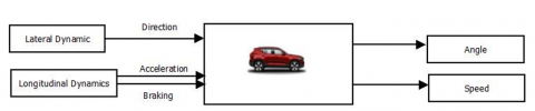
Dynamic modeling gives the relations between applied forces and movements. In the case of the vehicle, there is the longitudinal movement (longitudinal dynamics) and the lateral movement (lateral dynamics). The model of the system is shown in the following Figure 1.
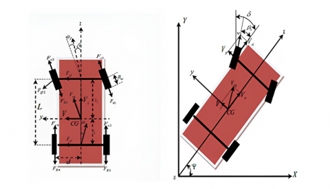
The Figure 2 shows the forces acting at the wheel-ground interface: In order to find the equations of the movements exerted on the vehicle, we adopt the following assumptions and laws:
Assumption 1: The road is considered flat (without tilt) and uniform (coating without defect). Its coating ensures good adhesion conditions (tar in dry weather).
Assumption 2: The acceleration of the vehicle (in traction and braking) is low enough that the movements of the suspensions are assumed to be negligible.
Assumption 3: The displacement of the vehicle is considered along the x, y axes, as well as a rotation around the vertical axis z.
Assumption 4: The rotation movement is a single degree of freedom that corresponds to yaw movement ψ. The other two degrees of freedom: roll and pitch are not taken into consideration (θ = 0, φ = 0).
Assumption 5: The center of gravity of the vehicle is confused with the origin of the reference mark linked to the vehicle (CG = 0).
Assumption 6: Considering the symmetry of the vehicle with its center of gravity CG we can note:
Assumption 7: Generally, the types of the front and rear axles are identical, so the stiffness Cf = Cr = C coefficient is identical
Figure 1. Modeling of the system
Figure 2. Projection of forces on axis (x, y)
The choice of vehicle model is based on assumptions related to its behavior within a convoy of vehicles. Failure to adhere to these assumptions does not guarantee the maintenance of a safe distance.
From the simplifications allowed by our assumptions and in the linearization around a turning angle δ considered small on the highway, we obtain the expressions of the dynamic model in a reference linked to the vehicle.
$\dot{V}_X=V_Y \dot{\Psi}+\frac{C}{M v} \frac{V_Y}{V_X}+\frac{L C}{2 M v} \frac{\dot{\psi}}{V_X} \delta$ (1)
$\dot{V}_Y=-V_X \psi+\frac{C}{M v} \delta-\frac{2 C}{M v} \frac{V_Y}{V_X}$ (2)
$\ddot{\psi}=\frac{L C}{2 J_v} \delta-\frac{L^2}{2 J_v} \frac{\dot{\psi}}{V_X}$ (3)
2.2 Control of inter-distance
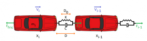
The main objective is to design a control strategy well adapted to control these inter-distances, in particular to control the longitudinal and lateral distances of each vehicle, based on an algorithm that implements a virtual impedance (a chain of spring-dampers) to impose the desired interaction effects between each pair of adjacent vehicles in Figure 3. Each vehicle is represented by its position $\vec{X}_i=\left(x_i, y_i\right)$, the mass of the vehicle is noted by mi:
Figure 3. Virtual spring-damping model
The physical quantities are listed in the Table 1.
Table 1. Definition of physical quantities
|
Lf |
Length between the front vehicle and the center of gravity |
|
FYf, FYr |
Lateral forces of pneumatic-road contact applied to the front and rear wheel respectively |
|
FXf, FXr |
Longitudinal forces of pneumatic-road contact applied to the front and rear wheel respectively |
|
VX |
Longitudinal speed |
|
VY |
Lateral speed |
|
r = $\dot{\psi}$ |
Yaw speed |
|
δ |
Tuning angle |
|
L |
Length between the two front and rear vehicles |
|
Lr |
Length between the rear vehicle and the center of gravity |
|
Rw |
The wheel radius |
|
FX |
The longitudinal force |
|
FY |
The lateral force |
|
λ |
The longitudinal sliding coefficient |
|
Mv |
The mass of the vehicle |
Vi−1, Vi: The speed of the front and rear vehicle respectively; K: Spring stiffness, C: Damping coefficient; D0: Empty length; Ff rot: The frictional force; D: The Safety distance; Xi−1, Xi: The position of the front and rear vehicle respectively; Fi−1, Fi: The front and rear damping-spring force applied to the vehicle. The inter-distance between the vehicles is given by:
$D=X_{i=1}-X_i$ (4)
The expressions of the forces applied to the vehicle are:
a) Spring force:
$F_{\text {spring }}=-K\left(D-D_0\right)$ (5)
b) Damping force:
$F_{\text {damping }}=-C \times D$ (6)
c) Damping force:
$F_{\text {fric }}=-C_1 \times X_i D=X_{i-1}-X_i$ (7)
At time t, we consider the relative distance D between two consecutive vehicles which is given by the following Eq. (8):
$D=\int\left(V_{i-1}-V_i\right) d t+D_{\text {initial }}$ (8)
Dinitial: represents the initial distance between the vehicles, at that moment t = 0. It should be noted that this model of the inter-distance is developed for the case of vehicles moving in a straight line, one behind the other.
$m_i \ddot{X}_l=F_{P I D}+F_{i-1}-F_i-F_{f r i c}$ (9)
3.1 Operational domain
To synthesize individual estimators of the nth derivative of the input signal X(t), the basic idea is to estimate only the coefficient xn(0) of the Taylor development of X(t). Let us ignore the noise for a moment. Assume that X(t) is analytic, then we can consider, without any loss of generality, the convergence of Taylor series.
$X(t)=\sum_{i=1}^N x^i(0) \frac{t^i}{i !}$ (10)
with N > n, the limit development of Taylor:
$x_n(t)=\sum_{i \geq 0}^N x^i(0) \frac{t^i}{i !}$ (11)
Satisfying the differential Eq. (12):
$\frac{d^{N+1}}{d t^{N+1}} x_n(t)=0$ (12)
In the operational area, which reads as:
$\begin{aligned} & s^{N+1} \hat{x}_N(s)=s^N \mathrm{x}(0)+s^{N-1} \mathrm{x}(0)+\cdots +s^{N-n} x^{(n)}(0)+x^N(0)\end{aligned}$ (13)
All $s^N x^{(i)}(0)$ terms are considered undesirable, for that it is enough to find a differential linear operator.
$\prod=\sum_{\text {finite }} Q_l(s) \frac{d^l}{d s^l}, \quad Q_l(s) \in C(s)$ (14)
Satisfying:
$\prod \hat{x}_N=Q_l(s) x^{(n)}(0)$ (15)
Remark:
Multiplying a differential operator by a rational function gives a cancellation function. We replace x(t) by the noisy measurement y(t), so the previous Eq. (14) becomes:
$Q(s) \tilde{x}_N^{(n)}(0)=\sum_{\text {finite }} Q_l(s) \frac{d^l}{d s^l} \hat{y}$ (16)
Note that Ql(s) and Q(s) are rational functions, f(t) and h(t) their impulse response, the operator d⁄ds corresponds to the multiplication by -t, the previous Eq. (16) becomes:
$f(t) \tilde{x}_N^{(n)}(0)=\sum_{\text {finite }} h_l(t-\alpha)\left(-1^l\right) \alpha^l y(\alpha) d \alpha$ (17)
3.2 Estimation of the punctual derivative
In all the following study we will use a particular family of derivatives called the anulators. A linear differential operator $П$ is said to be integral in finite form, if and only Ql(s) is in the form:
$Q_l(s)=\frac{1}{s} H_l \frac{1}{s}$ (18)
We consider the family of annulators considered below.
3.2.1 Lemma 1
For all k, $\mu \in N$ the differential operator
$\prod_{k, \mu}^{N, n}=\frac{1}{s^{N+\mu+1}} \frac{d^{n+k}}{d s^{n+k}} \frac{1}{s} \frac{d^{N-n}}{d s^{N-n}} s^{N+1}$ (19)
is a finite integral form of annulator associated with
$\varphi_{k, \mu, N}(s)=\frac{-1^{(n+k)}(n+k) !(N-n) !}{s^{\mu+k+N+n+2}}$ (20)
In the case where N = n the operational operator becomes:
$\prod_{k, \mu}^n=\frac{1}{s^{N+\mu+1}} \frac{d^{n+k}}{d s^{n+k}} s^n$ (21)
3.2.2 Theorem 1
Let $N, n$ and $\mu$ positive constants, where $N \geq n, q=N-n$, the $n^{\text {th }}$ estimate of $\tilde{x}^{(n)}(0 ; k ; \mu ; N)$, Taylor's expansion of order $N$ is particularly well expressed in the form:
3.3 Bias term minimization
3.3.1 Jacobi orthogonal polynomials
To begin with, recall that for a given signal and a positive integer the time domain analog of $\hat{v}=\frac{1}{s^\alpha} \frac{d^\beta}{d s^\beta} \hat{\mu}$.
Using the well-known Cauchy formula for repeated integration:
$v(t)=\frac{1}{(\alpha-1) !} \int_0^t(t-\tau)^{\alpha-1}(-1)^\beta \tau^\beta u(\tau) d \tau$ (23)
So we find the following result:
$\varphi_{k, u, n}(s) \cdot \tilde{x}_N^{(n)}=\prod_{k, u}^{n, N} \hat{y}$ (24)
$\tilde{x}^{(n)}(0)=\frac{S^{\mu+k+N+n+2}}{-1^{(n+k)}(n+k) !(N-n) !} \frac{1}{S^{\mu+n+1}} \frac{d^{n+k}}{d S^{n+k}} S^n \hat{y}$ (25)
3.3.2 Using Cauchy’s formula
We find in case = n:
$\begin{array}{r}\tilde{x}^{(n)}=\frac{(\mu+k+N+n+2) !}{(\mu+n) !(k+n) !} \int_0^T(T -\tau)^{\mu+n} \tau^{k+n} \gamma^{(n)}(\tau) d \tau\end{array}$ (26)
where n = 1:
$\begin{array}{r}\tilde{x}^{(n)}(0 ; k ; \mu)=\frac{(\mu+k+3) !}{(\mu+n) !(k+n) !} \int_0^1(1 -\tau)^{\mu+n} \tau^{k+n} y^{(n)}(\tau) d \tau\end{array}$ (27)
3.4 Estimated delay time
Corollary: let y(t) = x(t) + b(t)
$\tilde{x}^{(n)}(t ; k ; \mu) \approx x^{(n)}\left(t-\tau_1\right), \quad t \geq T$ (28)
$\tau_1=T \xi_1$ is the timedelay where $\xi_1=\frac{k+n+1}{\mu+k+2(n+1)}$
Similarly, we have the case of anti-causality
$\tilde{x}^{(n)}(t ; k ; \mu) \approx x^{(n)}\left(t+\tau_1\right), \quad t \geq T$ (29)
3.5 Reduce the effect of noise
We get from the integral by part of the Eq. (27) putting:
$\delta_{k, u, n}=\frac{(u+k+2 n+1)}{(u+n) !(k+n) !}$
$\begin{gathered}\tilde{x}^{(n)}(t ; k ; \mu)=\delta_{k, u, n} \int_0^1 \tau^{k+n}(1-\tau)^{\mu+n} x^{(n)}(T \tau) d \tau +\frac{(-1)^n \delta_{k, \mu, n}}{T^n} \int_0^1 \frac{d^n}{d \tau^n}\left\{\tau^{k+n}(1\right. \left.-\tau)^{\mu+n}\right\} b(T \tau) d \tau\end{gathered}$ (30)
The causality (k, u) is equivalent to the stability and the linear causality of an invariant time filter of the previous Eq. (30), we obtain:
$\begin{gathered}\tilde{x}^{(n)}(t ; k ; \mu)=\frac{(-1)^n \delta_{k, u, n}}{T^n} \int_0^1 \frac{d^n}{d \tau^n}\left\{\tau^{k+n}(1\right. \left.-\tau)^{\mu+n}\right\} y(t-T \tau) d \tau\end{gathered}$ (31)
3.6 Filter expression
First of all, let us recall that the numerical estimates are obtained as follows:
$\tilde{x}^{(n)}(T t ; k ; \mu ; N)=\int_0^1 g(\tau) y(t-T \tau) d \tau$ (32)
where,
$g(\tau)=\sum_0^q \lambda_1 h_{k+q-l, u+l}(\tau) d \tau$
The estimation time is $T=M T_s$. We use the trapezium method for the calculation of the following integral: $\int_0^1 f(t) d t \approx \sum_{m=0}^M\left(W_m f\left(t_m\right)\right)$.
Then we find:
$\tilde{x}^{(\mathrm{n})}\left(t_1 ; k ; \mu ; N\right) \approx x_l^n=\sum_{m=0}^M\left(W_m g_m y_{l-m}\right)$ (33)
With: $W_0=T_s / 2$ and $W_m=T_s, m=1, \ldots, M-1$.
Remark: The minimum estimator is calculated from N = n.
In order to improve the vehicle’s, inter-distance control, we propose an intelligent method based on the PI controller with an intelligent part that prevents the model’s behaviour based on previous measurements, it allows a better response in terms of uncertain additive noise. These can affect the behaviour of the system’s sensors, actuators, and other external actions that can affect the speed of the vehicles to be controlled.
4.1 Control strategy
Model-free control in the study [4] and its "intelligent" correctors have been invented to fill these gaps. The unknown global model is replaced by the ultra-local model:
$y^v=a+b u$ (34)
u, y variables refer to the control and output respectively, a represents coefficient estimated for each sampling session according to the inputs and outputs of the system and b a coefficient chosen according to the process to be controlled. We then obtain the Eq. (35) which is described mathematically in the form of the following inputs/outputs:
$E\left(y, \dot{y}, \ldots, y^{(a)}, u, \dot{u}, \ldots, u^{(b)}, d\right)=0$ (35)
d represents disturbances that are generally caused by external sources. The objective is to ensure the proper tracking [20] of trajectories even if the precise dynamics of the system are not required. For this approach. We must ensure the following hypothesis: "For all differential equations describing the system, there is a minimum integer m" such that at least locally, these equations verify the following Eq. (36):
$y^m=a+b u$ (36)
m is the same derivative chosen according to the designer (m is different from a of the equation). The differential Eq. (37) describing the input/output behaviour of a system is represented by:
$E\left(y, \dot{y}, \ldots, y^{(a)}, u, \dot{u}, \ldots, u^{(b)}\right)=0$ (37)
If, for $0<n<a, \frac{\partial E}{\partial y^n} \neq 0$, the implicit function theorem allows the Eq. (37) to be rewritten locally in the form:
$y^n=\xi\left(t, y, \ldots, y^{(n-1)}, y^{(n+1)}, \ldots, y^{(a)}, u, \ldots, u^{(b)}\right)$ (38)
By substituting this Eq. (38), applied over a very short time interval, with the following ultra-local model:
$y^v=F+\alpha u$ (39)
The constant $\alpha$ is a non-physical parameter, fixed by the operator.
$\begin{gathered}u(k)=\frac{-[F]_e}{\alpha}+\frac{y^{*(v)}(t)}{\alpha}+K_P e(t)+K_i+\int e(t) +K_D \frac{d}{d t} e(t)\end{gathered}$ (40)
$y^*$: is the reference trajectory of the output, obtained according to the rules of platitude control.
$y^{*(v)}$: is the derivative of the reference trajectory
$e=y-y^*$: is the tracking error
KP, Ki, KD: are the control gains.
The numerical value of F, which contains all the structural information of the system, is obtained in such a way as to avoid any algebraic looping due to the delay involved in the control sent to the system:
$[F]_e=\left[y^v(k)\right]_e-\alpha u(k-1)$ (41)
$\left[y^v(k)\right]_e$: refers to the estimate at the time "k".
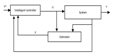
4.2 Algorithm
Figure 4. General principle of the model-free control
In the following, we will limit our study to mono-variable systems with minimal phase shift systems and in the case of $v=1$. In such case the intelligent-PI becomes:
$u=\frac{-F}{\alpha}+\frac{y^*}{\alpha}+K_P e+K_i \int e$ (42)
Where, y(t) is a signal that we want to estimate y in:
$F=[\dot{y}(k)]_e-\alpha u(k-1)$ (43)
Let’s summarize the intelligent-PI algorithm into Eqs. (44)-(46):
$u=\frac{-F}{\alpha}+\frac{y^*}{\alpha}+K_P e+K_i \int e$ (44)
$F=y^*(k)-\alpha u(k-1)$ (45)
$\begin{aligned} & y^*\left(k, T_e\right) =\frac{-3 !}{\left(n_P-T_P\right)^3} \sum_{i=0}^{n_P}\left(n_P-2 i\right) T_P \times y\left((k-i) T_P\right)\end{aligned}$ (46)
This algorithm synthesizes model-free control as shown in Figure 4. The comparison between the classic controller and the intelligent corrector is based on the work in the study [9, 16].
We consider a vehicle model with the following characteristics: a mass of 1300 kg and viscous friction of 180. The tuning coefficients of the PI controller are as follows:
Kp=1 and Ti=0.1
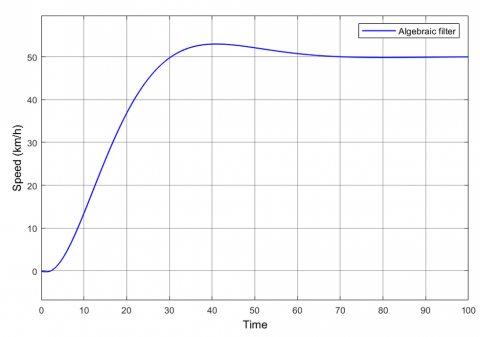
The result of the simulation of the model-free speed control in the presence of an algebraic filter is presented in the following Figure 5.
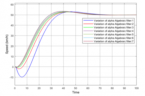
The Model-free control based on iPI controller has been tested for several values of the α parameter.
Considering that adjusting the parameters of the model-free control is easier since the parameters of the PI remain unchanged, only the alpha parameter can stabilize the system. We observe from the Figure 6 that increasing the value of the alpha coefficient varies proportionally with the speed and response time of the system, and slightly increases stability, which is directly linked to the algebraic filter, especially in the presence of noise.
To obtain the best results, the values of α are: 0.1 < α < 1, for speed control. In our case, we used α = 0.45 for the speed control.
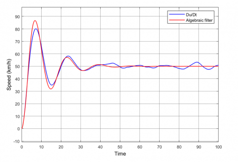
In order to demonstrate the effectiveness of our approach, a comparative simulations between the algebraic filter and the simple derivative are given in Figures 7, 8 and 9.
Figure 5. Model-free speed control with algebraic filter
Figure 6. Tuning coefficient in model-free control
Figure 7. Comparison of model-free control between simple derivative and algebraic filter
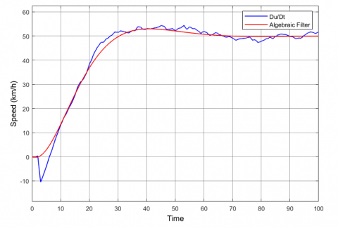
Figure 8. Variation of speed in the presence of disturbances
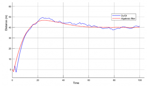
Figure 9. Variation of distance in the presence of disturbances
Response time for (simple derivative)= 26 seconds.
Response time for (Algebraic filter)= 23 seconds.
Error rates for (simple derivative)= 2.4%.
Error rates for (Algebraic Filter)= 0.2%.
The algebraic filter enables the model-free control system to better respond to system variations and maintain robust control performance even in the presence of noise. It acts as a preprocessing step by removing undesirable noise from the input of the model-free control system, thereby improving control quality by reducing the adverse effects of noise.
The purpose of this work is to ensure a safe distance in a vehicle convoy, using intelligent inter-distance control techniques. In order to achieve this objective, we have developed an iPI controller for speed and distance. The estimation component of the model-free control aims to anticipate the model’s behaviour using measurements from previous instances. The advantage of this approach lies in the ease of adjusting the regulator parameters with a single coefficient. This control also includes a derivation component, for which we conducted a comparative synthesis between a simple derivative and an algebraic filter. The latter appears to be more effective because it filters uncertain additive terms, thereby enhancing control robustness. In order to complete the study of this project, several other factors must be taken into account, including with regard to vehicle control and models, the dynamic model used can be extended to take into account slippages, which can give a more accurate response. Adopt the case of a turning situation where the vehicle follows a circular trajectory of finite radius. In perspective, our next work will consider nonlinearities by proposing a model-free controller based on fuzzy logic. Furthermore, we will be able to integrate an intelligent system capable of detecting driver fatigue using AI and helping to prevent accidents caused by a lack of attention or falling asleep at the wheel. Furthermore, with AI, we will be able to detect and identify anomalies in advance from sensors.
[1] Kareem, E.I.A., Hoomod, H.K. (2022). Integrated tripartite modules for intelligent traffic light system. International Journal of Electrical and Computer Engineering (IJECE), 12(3): 2971-2985. https://doi.org/10.11591/ijece.v12i3.pp2971-2985
[2] Mazenc, F., Niculescu, S.I., Bekaik, M. (2013). Stabilization of time-varying nonlinear systems with distributed input delay by feedback of plant’s state. In 2011 50th IEEE Conference on Decision and Control and European Control Conference, Orlando, FL, USA, pp. 7605-7610. https://doi.org/10.1109/CDC.2011.6160191
[3] El-Nagar, A.M., El-Bardini, M., EL-Rabaie, N.M. (2014). Intelligent control for nonlinear inverted pendulum based on interval type-2 fuzzy PD controller. Alexandria Engineering Journal, 53(1): 23-32. https://doi.org/10.1016/j.aej.2013.11.006
[4] Molina, J.J.M. (2005). Commande de l’inter-distance entre deux véhicules. Doctorat dissertation. Institut National Polytechnique de Grenoble-INPG.
[5] Akki, M. (2010). Commande de l’inter distances dans un convoi de véhicules autonomes par l’imposition d’impédances virtuelles d’interaction. Doctoral dissertation. Université du Québec à Trois-Rivières.
[6] Khalyasmaa, A., Matrenin, P., Eroshenko, S. (2022). Inappropriate machine learning application in real power industry cases. International Journal of Electrical and Computer Engineering (IJECE), 12(3): 3023-3032. https://doi.org/10.11591/ijece.v12i3.pp3023-3032
[7] Chaïbet, A. (2006). Contrôle latérale et longitudinale pour le suivi de véhicule. Doctoral dissertation. University of Evry-Val-d’Essonne.
[8] Badji, B. (2009). Caractéristique du comportement non linéaire en dynamique du véhicule. Doctoral dissertation. De l’automatique, Univ Belfort-Montbéliard.
[9] Venture, G. (2003). Identification des paramètres dynamiques d’une voiture. Doctorat dissertation. Ecole Centrale de Nantes (ECN); Université de Nantes.
[10] d'Andréa-Novel, B., Boussard, C., Fliess, M., El Hamzaoui, O., Mounier, H., Steux, B. (2010). Commande sans modèle de vitesse longitudinale d’un véhicule électrique. In Sixième Conférence Internationale Francophone d'Automatique (CIFA 2010), Nancy, France.
[11] Besancon-Voda, A., Gentil, S. (1999). Régulateur PID analogiques et numériques. Techniques de l'ingénieur. Informatique industrielle, 2(R7416): R7416-1.
[12] Mhawesh, M.A. (2021). Performance comparison between variants PID controllers and unity feedback control system for the response of the angular position of the DC motor. International Journal of Electrical and Computer Engineering (IJECE), 11(1): 802-814. https://doi.org/10.11591/ijece.v11i1.pp802-814
[13] Thampi, P., Sahridayan, M., Gopal, R. (2022). Modeling and analysis of field-oriented control based permanent magnet synchronous motor drive system using fuzzy logic controller with speed response improvement. International Journal of Electrical and Computer Engineering (IJECE), 12(6): 6010-6021. https://doi.org/10.11591/ijece.v12i6.pp6010-6021
[14] Trujillo, O.A., Toro-García, N., Hoyos, F.E. (2019). PID controller using rapid control prototyping techniques. International Journal of Electrical and Computer Engineering (IJECE), 9(3): 1645-1655. http://doi.org/10.11591/ijece.v9i3.pp1645-1655
[15] Jha, S.K., Gaur, P., Yadav, A.K. (2016). Various intelligent control techniques for attitude control of an aircraft system. In 2016 3rd International Conference on Computing for Sustainable Global Development (INDIACom), New Delhi, India, pp. 2476-2480.
[16] Kim, J.W., Oh, C.Y., Chung, J.W., Kim, K.H. (2017). Brain emotional limbic-based intelligent controller design for control of a haptic device. International Journal of Automation and Control, 11(4): 358-371. https://doi.org/10.1504/IJAAC.2017.087041
[17] Novel, A., Fliess, B., Join, M., Mounier, C. (2010). A mathematical explanation via intelligent PID controllers of the strange ubiquity of PIDs. In 18th Mediterranean Conference on Control and Automation, MED'10, Marrakech, Morocco, pp. 395-400. https://doi.org/10.1109/MED.2010.5547700.
[18] Fliess, M., Join, C. (2013). Model-free control. International Journal of Control, 86(12): 2228-2252. https://doi.org/10.1080/00207179.2013.810345
[19] Mirwald, J., Ulttsch, J., de Castro, R., Brembeck, J. (2021). Learning-based cooperative adaptive cruise control. Actuators, 10(11): 286. https://doi.org/10.3390/act10110286
[20] Chater, E.A., Housny, H., El Fadil, H. (2022). Adaptive proportional integral derivative deep feedforward network for quadrotor trajectory-tracking flight control. International Journal of Electrical and Computer Engineering (IJECE), 12(4): 3607-3619. http://doi.org/10.11591/ijece.v12i4.pp3607-3619