Zixuan Zhang![]() | Hirosuke Horii*
| Hirosuke Horii*![]() | Nobutaka Tsujiuchi
| Nobutaka Tsujiuchi![]() | Akihito Ito
| Akihito Ito![]()
© 2024 The authors. This article is published by IIETA and is licensed under the CC BY 4.0 license (http://creativecommons.org/licenses/by/4.0/).
OPEN ACCESS
This study explores a methodology for mapping the 3D spatial information of evacuation routes, aiming to acquire lightweight data to enhance the flexibility of evacuation route development. Utilizing 3D-LiDAR (Light Detection and Ranging) technology, we integrated an Inertial Measurement Unit (IMU) with an existing algorithm to compensate for motion distortion, thereby increasing the mapping accuracy of interior spaces characterized by a paucity of structural features. Given the extensive volume of point cloud data generated by LiDAR, which is impractical for direct application in evacuation route mapping, we categorized the data into local and global maps. This paper presents a strategy to minimize the data volume necessary for generating optimized evacuation route maps, employing the Octomap data format for efficient global map storage. This approach not only addresses the challenges of handling large datasets but also contributes to the development of more accurate and user-friendly evacuation planning tools.
evacuation guidance, Laser Odometry and Mapping (LOAM), Octomap, self-motion distortion, solid-state 3D-LiDAR
Japan is one of the world’s most earthquake-prone countries. Japan and its surrounding areas experience roughly a tenth of all earthquakes that occur in the world [1]. The critical role of rescue robots in such scenarios, specifically in path planning and navigation to reach trapped or injured individuals swiftly, becomes indispensable. For example, during the 2011 Tohoku earthquake and tsunami [2], the rapid deployment of rescue robots could have facilitated quicker access to affected areas, showcasing the immediate need for advancements in robotics for disaster response [3].
Such natural disasters rely on escape routes established based on advanced evacuation plans. However, smooth, safe, and efficient evacuations are greatly complicated if only a preliminary evacuation plan is relied upon because the actual situations change very rapidly: traffic obstructions from fires collapsed buildings along evacuation routes, and traffic congestion from fleeing evacuees. Recent studies [4, 5], including our team's prior research [6], have demonstrated through simulations the potentially unsafe conditions caused by the congregation and stalling of individuals during disasters. This highlights the importance of real-time path planning to mitigate risks and ensure the safety of evacuees.
Our research is grounded in the realization that disaster scenarios are highly dynamic, with people crowding and new obstacles frequently emerging making the pre-existing evacuation plans quickly outdated. This unpredictability necessitates the development of an evacuation guidance support robot capable of adapting to the ever-changing environment. Our project’s ultimate goal is to develop an evacuation guidance support robot that can search for evacuation routes during disasters, observe damage and evacuation states, and formulate more flexible evacuation routes tailored for specific situations [7]. For an evacuation support robot to cope with severe conditions during a disaster, such sensor information as LiDAR, camera images, and ultrasonic waves must be integrated to observe and comprehend the overall situation. This study discusses the use of LiDAR in this.
We explored the application of Laser Odometry and Mapping (LOAM) [8] as a method for capturing and reducing 3D spatial information of evacuation routes, with an emphasis on minimizing the volume of data acquired. With the ability to provide long-range, highly accurate 3D measurements of the surrounding environment, 3D-LiDAR is becoming an essential sensor in many robotic applications, such as autonomous driving vehicles [9], drones [10], surveying, and mapping [11, 12]. The capability of 3D-LiDAR to scan spaces in three dimensions addresses the limitation inherent in 2D-LiDAR. Specifically, 2D-LiDAR is constrained to scanning solely at the elevation at which it is positioned, potentially leading to the omission of crucial spatial information. In contrast, 3D-LiDAR offers a comprehensive spatial representation, eliminating such blind spots.
We collected 3D data using DJI Livox 3D-LiDAR [13], which represents a new class of solid-state LiDAR featuring non-repetitive scanning patterns, garnering increased attention and development. Since solid-state LiDAR can be massively produced, such high-performance and extremely low-cost LiDAR have the potential to promote or radically change the robotics industry [14]. Despite their cost and reliability superiority, as well as potential performance advantages compared with conventional mechanical spinning LiDAR, solid-state LiDAR offers many new features that significantly challenge LiDAR navigation and mapping. These features include (taking the Livox MID-40 LiDAR as an example) a small FOV (field of view), irregular scanning patterns, non-repetitive scanning, and motion blur [15].
The Loam-Livox software suite was specifically designed for processing data from the Livox LiDAR [16]. Its algorithm performs real-time mapping using only LiDAR data. Due to the limitations of the DJI Livox Mid-40 LiDAR itself and the fact that the Loam-Livox algorithm maps based on a single data source, the risk of drift is high in scenes where feature points are not abundant (degenerate scenes).
This study further optimizes mapping methods with this software package, which we use in conjunction with an IMU, which compensates for self-motion distortion during LiDAR scans and reduces the occurrence of indoor drifts. The map derived from LiDAR through SLAM (Simultaneous Localization and Mapping) is divided into local and global maps, and an Octomap [17] representation scheme is introduced to reduce the data volume.
2.1 Self-motion distortion
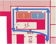
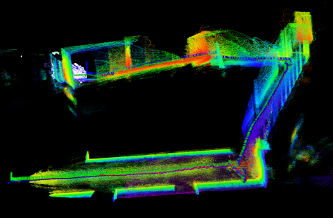
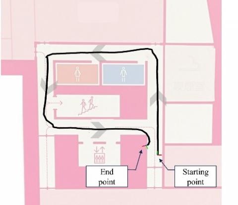
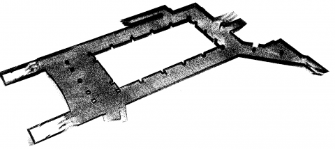
In previously proposed Loam-Livox software packages, motion drift generally occurs in indoor scenes, that is, in a degeneration environment with fewer feature points. When we conducted experiments on the basement floor of a building (Figure 1), the probability of such a drift problem was high during turns in the corridor by the LiDAR. LiDAR followed a nearly rectangular path along the corridor, eventually returning near the starting point. We used the LiDAR data obtained from the scan to construct a 3D model (Figure 2).
Figure 1. Schematic diagram of floor
Figure 2. Constructed point cloud map of floor
The odometry data representing the scanned path were output (Figure 3). From the scan’s start, -13.4 m drift occurred on the X-axis, 3.5 m on the Y-axis, and -11.9 m on the Z-axis. We analyzed the cause of this drift. Indoor scenes (Figure 4) often suffer from too many similar planar features (especially in hallways) due to unchanging walls. When used for matching, these planar features cause misrecognition and drift in the odometry.
(a) XYZ Third person perspective
(b) XOY top view
Figure 3. Odometry path of corridor
Figure 4. Example of excessive similar planar features
Another reason for the drift is that the FOV of a solid-state LiDAR is narrower than a mechanical LiDAR. For example, the FOV of the Livox Mid-40 used in this experiment was only 38.4°.
For most LiDARs, although the laser is transmitted and received quickly, each point from which the point cloud is comprised is not generated at the exact moment. In general, we output data accumulated within 100 ms (corresponding to a typical value of 10 Hz) as one frame of the point cloud. If the absolute location of the LiDAR body or the body where it is mounted changes during this 100 ms, the coordinate system of each point in this frame point cloud will be changed. Intuitively, this frame of the point cloud data becomes "distorted" and will not correspond to the detected environmental information. This resembles taking a photo: if your handshakes, the photo will be blurry. This is the self-motion distortion of LiDAR.
In particular, when turning, errors occur in the positional relationship between the point clouds in the same frame owing to self-motion distortion. Errors also exist in the projection of the feature points at the same position in different frames. This situation reduces the number of reliable feature points, causing odometry that is prone to drift during LiDAR turns.
2.2 Self-motion distortion removal by IMU
To mitigate these challenges, we introduced an IMU to our experimental setup, aiming to correct for self-motion distortions. The integration of IMU data, sampled at a higher frequency of 200 Hz compared to the LiDAR's 10 Hz, allows for real-time adjustment of the LiDAR data, compensating for the device's movements and rotations. The confluence of LiDAR and IMU data stands as a cornerstone of our methodological approach, facilitating real-time adjustments to the LiDAR's positional data.
First, the initial phase involves the synchronization of LiDAR and IMU data, coupled with the derivation of a transformation matrix. This matrix serves to reconcile the LiDAR and IMU coordinate systems, accommodating both rotational and translational movements of the LiDAR device. The establishment of this matrix is critical for the subsequent alignment of point cloud frames with the IMU's temporal data, ensuring accuracy in environmental representation.
We must contend with three central coordinate systems: global, IMU, and LiDAR. A global coordinate system generally considers the starting point as the origin, whereas an IMU coordinate system changes from moment to moment and is purely an estimate of the IMU data. If the IMU coordinate system is known, the LiDAR coordinate system is also known. Therefore, a transformation matrix must be created to place both sets of data in the same coordinate system [18]. The positive direction is counterclockwise, rotating around the X-axis by α, then around the Y-axis by angle β, and finally around the Z-axis by angle γ. Rotation matrix R is given by Eq. (1). We use Eq. (2) for brevity:
$R=R_z R_y R_z=\left[\begin{array}{ccc}\cos \beta \cos \gamma & \sin \alpha \sin \beta \cos \gamma-\cos \alpha \sin \gamma & \cos \alpha \sin \beta \cos \gamma+\sin \alpha \sin \gamma \\ \cos \beta \sin \gamma & \sin \alpha \sin \beta \sin \gamma+\cos \alpha \cos \gamma & \cos \alpha \sin \beta \sin \gamma-\sin \alpha \cos \gamma \\ -\sin \beta & \sin \alpha \cos \beta & \cos \alpha \cos \beta\end{array}\right]$ (1)
$R=\left[\begin{array}{lll}R_{11} & R_{12} & R_{13} \\ R_{21} & R_{22} & R_{23} \\ R_{31} & R_{32} & R_{33}\end{array}\right]$ (2)
By measuring the relationship between the distance and angle, transformation matrix ${ }^I T_L$ from the LiDAR coordinates to the IMU coordinates becomes
${ }^I T_L=\left[\begin{array}{cccc}R_{11} & R_{12} & R_{13} & T_x \\ R_{21} & R_{22} & R_{23} & T_y \\ R_{31} & R_{32} & R_{33} & T_z \\ 0 & 0 & 0 & 1\end{array}\right]$ (3)
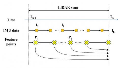
Following matrix establishment, the correction of each point's motion within the LiDAR frame is executed through an error back-propagation method (Figure 5). This process entails pinpointing the IMU data correlating with the start and end times of each LiDAR frame. By applying the transformation matrix to adjust the point cloud data accordingly, distortions attributable to device movement are meticulously corrected.
Integral to this correction process is the comprehensive integration of IMU data throughout the LiDAR scanning cycle. This step involves calculating frame velocity, displacement, and angular velocity integrals, thereby facilitating the precise projection of each point to its accurate position within the global coordinate framework.
To elaborate on the computational steps involved in this process, Algorithm 1 presents a simplified pseudocode, summarizing the core logic behind the self-motion distortion correction using IMU data.
Figure 5. Removing self-motion distortions with back-propagation
|
Algorithm 1 Self-Motion Distortion Removal using IMU Data |
|
Input: LiDAR scans, IMU data Output: Corrected point cloud 1. Initialize Global, IMU, and LiDAR Coordinate Systems 2. Calculate Transformation Matrix ${ }^I T_L$ for aligning IMU and LiDAR coordinate systems 3. for each scan in LiDAR scans do 4. for each frame in scan do 5. $T_{\text {start }}, T_{\text {end }}$ = Get IMU timestamps for frame 6. Accel corrected = Remove gravity influence from IMU data between $T_{\text {start }}$ and $T_{\text {end }}$ 7. Calculate Rotation Matrix and Displacement from accel corrected 8. for each point in frame do 9. Adjust point position using Transformation Matrix, Velocity, and Displacement 10. Project adjusted point into final frame position under LiDAR coordinate system 11. end for 12. end for 13. Combine adjusted frames into corrected point cloud 14. end for 15. |
Regarding the error back-propagation method, in detail, first using LiDAR data, locate the IMU data for the start time $T_{k-1}$ and end time $T_k$ of a frame. As the LiDAR's timing might not always align precisely with the IMU's timing, it is possible to find the nearest IMU timestamp. After removing the influence of gravity on the acceleration from each frame's IMU data, the actual acceleration of the IMU is obtained.
The LiDAR’s frequency (10 HZ) is much lower than that of the IMU (200 HZ). One cycle (100 ms) of point cloud data generates approximately 20 IMU of data. Taking the angular velocity in one direction as an example, the IMU of data is integrated in Eqs. (4) and (5):
$\alpha_t=\frac{\omega_{t 0}+\omega_t}{2}\left(t-t_0\right)$ (4)
$\alpha=\sum_{i=0}^{n-1} \alpha_i$ (5)
where, $\alpha_t$ is the angular change at time $t$ relative to previous time $t_0, \omega_{t 0}$, and $\omega_t$ are angular velocities at the corresponding times, and n is the IMU data. The IMU rotation angle within one cycle is obtained by repeating the integration and accumulation in this manner.
As in the above example, in Figure 5, the IMU data in $I_1 \sim I_k$ are integrated to obtain the frame velocity, the displacement, and angular velocity integrals. Based on the integration results, LiDAR data $P_j$ at any time in this frame are back-calculated into transformation matrix ${}^{I_k}T_{I_j}$ for end time $P_k$.
Each point belonging to time $T_k \sim T_{k-1}$ is projected onto the LiDAR coordinate system at the end time of the frame in question. The point cloud from the coordinate transformation becomes
${ }^{{ }^L k} P_{f_i}={ }^I T_L^{-1 I_k} T_{I_i}{ }^I T_L{ }^{L j} P_{f_j}$, (6)
where, ${ }^{L j} P_{f_j}$ and ${ }^{L_k} P_{f_j}$ are the point clouds at times j and k in frame f of the LiDAR coordinate system;
${ }^I T_L$ is the transformation matrix from the LiDAR coordinates to the IMU coordinates, and;
${ }^{{I}^k} T_{I_j}$ is the transformation matrix from the IMU coordinates at times j to k.
In this way, each point in the frame is projected under the LiDAR coordinate system at the final time to correct for such self-motion distortions as rotation in the LiDAR data.
3.1 Data filter
The obtained point cloud data were processed using the following three primary filters:
(1) A radius outlier removal filter [19] removes the outliers when the number of people within a specific search radius is fewer than a given quantity. This method has a good removal effect on some floating isolated or invalid points in the original point cloud data.
(2) A conditional removal filter, based on such conditions as point coordinates (x, y, z), removes or retains values for a given spatial range. The point cloud data are filtered based on the actual size of the scene and the height that makes sense of the navigation. This effectively reduces the amount of data required to retain just the meaningful points for generating a navigation map.
(3) A ground filter searches for and removes the ground surfaces based on the height, the tilt angle, and other parameters. It processes large contiguous planes with low heights and small horizontal undulation angles. These points are stored as ground-point clouds. Issues other than the ground-point cloud are used to generate navigation maps. If the original point cloud data, including the ground, are used as they are, the ground will also be recognized as an obstacle, and the entire map will be covered.
These processes produce point cloud data with noise and are ground-removed at a specific altitude. The resulting data are stored as a map in a 3D map called Octomap.
While filtering and storing the data in the Octomap, the 3D map is divided into ground and non-ground portions. The latter is cropped to an appropriate height and projected onto the XOY plane, producing a 2D map with three-dimensional occupancy information for planning evacuation routes.
3.2 Data storage
SLAM’s purpose is twofold: to estimate a robot's trajectory and to create an accurate map. Maps can be represented in various ways, including as feature points, grids, or topological depictions.
The map format used for LiDAR SLAM is primarily a point cloud map, which stores such information as spatial point coordinates and reflection intensity. However, this format suffers from two obvious flaws.
(1) The map format needs optimization for efficiency. Owing to their high-fidelity characteristics, point cloud maps inherently encapsulate an extensive range of details, thereby producing datasets of considerable magnitude. Post-filtering, the resultant PCD files, which serve as the primary data storage medium, still necessitate substantial storage capacity. This concern transcends mere physical storage implications; it profoundly impacts data transfer latency, computational processing velocities, and the efficacy of real-time operations. Importantly, not all captured details are universally relevant across applications. For instance, the granularity of point cloud maps can lead to the inclusion of inconsequential anomalies such as subtle carpet textural variances or minor wall imperfections. In numerous application scenarios, these superfluous details neither augment the map's utility nor its interpretability, but rather exacerbate storage demands. Consequently, there emerges an unequivocal imperative to refine and recalibrate the format, ensuring it retains only indispensable information, thus promoting optimized storage and expedited computational processing.
(2) Navigational Impediments in Point Cloud Maps: One of the principal objectives of a map within robotic applications is to facilitate effective navigation, guiding an autonomous agent from one point to another. However, the inherent structure of point cloud maps poses significant challenges in this regard. These maps, in their raw format, do not provide explicit delineations between navigable and non-navigable regions. Consequently, for a robot to achieve comprehensive and safe navigation, it requires more than the mere spatial data present in a point cloud.
Octree [20] is a method of dividing a three-dimensional space into eight recursive blocks, each of which is called an octant. Each block contains a number that describes whether it is occupied. In the simplest case, it can be represented as either 0 or 1. Typically, the probability of being occupied is expressed as a number between 0 and 1.
Octomap’s advantage is that it is a complete 3D model that is updatable and compact. If all the leaf nodes are occupied, unoccupied, or undetermined, their parent nodes can be cut. In other words, unless a particular need exists for a more detailed structure description (leaf nodes), coarse block information (parent nodes) is sufficient.
Octomap resolves the noise and movement effects on the map by providing a probabilistic representation of the current node state. $t=1, \ldots, T$, the observed data are $z_1, \ldots, z_T$, and the information recorded by the $n$-th leaf node is represented in Eq. (7):
$P\left(n \mid z_{1: T}\right)=\left[1+\frac{1-P\left(n \mid z_T\right)}{P\left(n \mid z_T\right)} \times \frac{1-P\left(n \mid z_{1: T-1}\right)}{P\left(n \mid z_{1: T-1}\right)} \times \frac{P(n)}{1-P(n)}\right]^{-1}$. (7)
Applying the following logit transformation of Eqs. (7) to (8), we obtain Eq. (9):
$p=\log it^{-1}(\alpha)=\frac{1}{1+\exp (-\alpha)}$, (8)
$L(n)=\log \left[\frac{p(n)}{1-p(n)}\right]$. (9)
Converting the solution in the probability space into real coordinate space yields Eq. (10):
$\mathrm{L}\left(n \mid z_{1: T}\right)=\mathrm{L}\left(n \mid z_{1: T-1}\right)+\mathrm{L}\left(n \mid z_T\right)$. (10)
In other words, newly scanned information is directly added to the existing data. When using a 3D map for navigation, a threshold value is set for occupancy probability $P\left(n \mid z_{1: T}\right)$. Voxels that reach this threshold are considered occupied. Otherwise, they are deemed vacant, and two discrete states are defined.
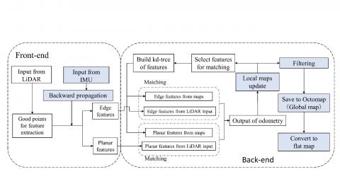
As depicted in Figure 6, the maps are categorized into local and global types. The former focuses on nearby feature point information, while the latter encompasses every point collected during the execution of SLAM. Our SLAM system adeptly combines local and global mapping to bolster real-time localization and comprehensive environmental modeling. Crucially, this integration is essential for realizing high-precision mapping, all while efficiently managing the computational load.
Local Mapping Strategy: Constructed in real-time from LiDAR data, local maps provide detailed information on the immediate vicinity's feature points. These maps are dynamically refreshed as the robot traverses the environment, guaranteeing updates at a high frequency that is critical for prompt pose estimation and swift adaptation to environmental changes.
Global Mapping Integration: Compiling every data point acquired through the SLAM process, the global map forms an exhaustive and intricate model of the environment. Although the global map's comprehensive nature offers an extensive spatial context, direct positioning within this map requires significant computational resources due to its data volume. To enhance system performance, updates to the global map occur at lower frequencies, effectively minimizing the computational demand.
Combining Local and Global Maps: The synergy between local and global maps is established through a filtration process that seamlessly integrates real-time local map updates into the global map structure. This process involves:
(1) Filtering: A selection of the most pertinent features from the local maps is filtered for matching. This step ensures the conservation of computational resources by focusing on the most relevant data points for global map updates.
(2) Saving to Octomap: The filtered local maps are then methodically incorporated into the Octomap, which serves as our global map repository. This process is designed to maintain the global map's continuity and accuracy over time.
(3) Conversion to a Flat Map: For practical applications, such as evacuation route planning, the global map's detailed three-dimensional information is converted into a more accessible flat map. This conversion involves projecting the processed global map data onto the XOY plane, resulting in a 2D representation that retains critical occupancy information.
The combination strategy ensures that the system maintains a real-time understanding of the environment through local maps while gradually building a comprehensive global map that encapsulates the entirety of the scanned area. This approach enables the system to provide accurate navigation and mapping capabilities essential for applications that require precise environmental awareness and path planning, such as in the context of disaster response or autonomous navigation.
Figure 6. System flow chart
4.1 Experiment that removes self-motion distortion
Next, we validated our algorithms and systems. An NVIDIA Jetson AGX Xavier was used in the experiments. The Jetson AGX Xavier is the world's first computer designed for autonomous machines, and the performances are needed for next-generation robots.
We used a WIT Motion WT901C IMU module. WT901C is an IMU sensor called the Attitude and Heading Reference System (AHRS), which measures the angle, angular velocity, acceleration, and magnetic field along three axes.
We used a 3D printer to create a container with the necessary hardware, including a Livox Mid-40 and a Jetson AGX Xavier for indoor and outdoor measurements.
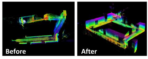
To evaluate the self-motion distortion when using the IMU, we rescanned the previously scanned basement floor of a building, an area wherein odometry drift had been observed, and compared the obtained results with those in Section 2. The constructed 3D model is shown in Figure 7.
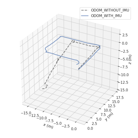
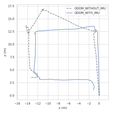
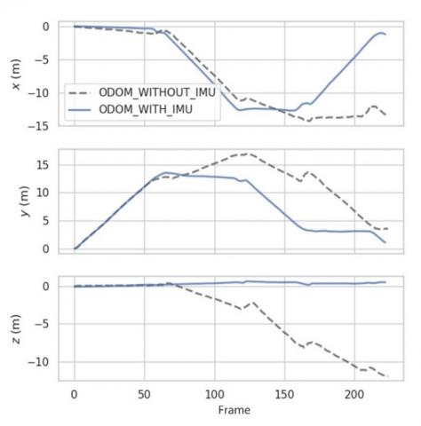
The odometry data representing the scanned path were output, as shown in Figure 8, and Figure 9 shows the change of the coordinates with an increasing frame number in each XYZ axis. The dotted line shows the data without the IMU, and the solid line shows the data after the self-motion distortion correction.
Figure 7. Comparison of constructed point cloud images
(a) XYZ Third person perspective
(b) XOY top view
Figure 8. Odometry path of basement floor
Our experimental results show that the algorithm more effectively corrects the self-motion distortion than the original Livox-Loam algorithm. In particular, no drift occurred during the rotation. All the rotation angles were close to 90°. The odometry returned near the starting point, an outcome that agrees with the experimental results (the starting and ending points do not coincide exactly). The odometry path is projected onto a map (Figure 10). Although some errors remained, the map’s accuracy showed a good fit.
Figure 9. Odometer data on X-, Y-, and Z-axes
Figure 10. Projection of odometry path on map
The endpoint coordinates show the following displacements from the starting point of the scan: -1.165 m on the X-axis, 1.108 m on the Y-axis, and 0.52 m on the Z-axis. The error was significantly reduced compared to the data without IMU: -13.4 m on the X-axis, 3.5 m on the Y-axis, and -11.9 m on the Z-axis.
Our investigation centers on the utilization of Solid-State LiDAR, integrated with an Inertial Measurement Unit (IMU), to enhance the mapping accuracy in such challenging environments. The crux of this method lies in its ability to compensate for the inherent indoor scene degradation through sophisticated data processing techniques, which correct self-motion distortion and significantly improve mapping fidelity. The methodology's efficacy is demonstrated through a comparative analysis of the Z-axis coordinate data, obtained from scans performed across the same floor level, thereby ensuring that the Z-axis coordinates are expected to remain constant, highlighting the algorithm's ability to maintain consistent height measurement despite the dynamic indoor environment.
The comparative analysis (Table 1) reveals that the algorithm incorporating IMU data exhibits superior performance in maintaining the integrity of the Z-axis measurements, as evidenced by the mean and standard deviation values of the Z-axis coordinates. Specifically, the mean Z-axis coordinate obtained with IMU integration (0.306158 meters) starkly contrasts with that derived from the Loam-Livox software without IMU assistance (-3.8111 meters), indicating a marked improvement in vertical axis stability and accuracy. Furthermore, the standard deviation with IMU (0.194372) is significantly lower than that without IMU (4.148744), demonstrating the enhanced precision and robustness of our method in mapping the horizontal plane.
This comparative analysis not only validates the effectiveness of integrating Solid-State LiDAR with IMU for indoor mapping but also highlights the algorithm's ability to navigate and accurately map spaces where conventional methods may falter due to feature degradation or environmental uniformity. Such a detailed quantitative analysis reinforces the novelty and utility of our approach in advancing robotic navigation and mapping technologies, especially in indoor degradation scene compensation.
Table 1. Z-axis coordinate data analysis
|
Our Method |
Loam-Livox |
|
|
Average |
0.306158 |
-3.8111 |
|
Standard error |
0.012987 |
0.2772 |
|
Median |
0.35587 |
-2.29935 |
|
Standard deviation |
0.194372 |
4.148744 |
|
Dispersion |
0.037781 |
17.21208 |
|
Range |
0.72491 |
12.36419 |
|
Minimum |
-0.08432 |
-11.9262 |
|
Maximum |
0.640587 |
0.437986 |
|
Total |
68.57932 |
-853.686 |
|
Number of data |
224 |
224 |
4.2 Experiment of Octomap algorithm
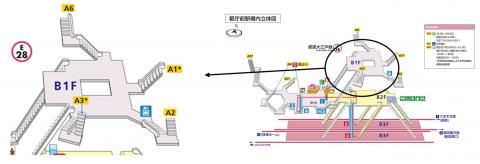
We conducted experiments using the Octomap algorithm to create a 2D map of a subway station’s (Figure 11) point cloud data. The point cloud data for this station is sourced from a public dataset provided by the Tokyo Metropolitan Government [21]. As detailed in Section 3, the station’s PCD file (Figure 12) was converted to an Octomap file, saved in different resolution settings, and the amount of data, file size, etc. were recorded.
We tested the impact of different resolutions on the file size reduction using Octomap. The higher the resolution, the smaller is the littlest block, and intuitively the map can be displayed more finely. We set six conditions (Figure 13) under resolutions of 0.2, 0.4, and 0.6 m. The experiments were conducted separately with and without the ground, and we recorded the number of data, file size, etc. The experiment results are shown in Table 2.
Figure 11. Subway station’s 3D map
Figure 12. PCD file of subway station
Figure 13. Octomap tested in six different conditions
Table 2. Test that converted PCD file to Octomap file
|
Ground |
No. |
Resolution |
Conversion Time [s] |
Points |
File Size [Mb] |
Ratio to PCD File |
|
|
PCD file |
990,768 |
27.5 |
100.0% |
||||
|
Octomap file |
Remove ground points |
➀ |
0.2 |
24 |
361,456 |
10.23 |
37.2% |
|
➁ |
0.4 |
21 |
73,454 |
2.08 |
7.6% |
||
|
➂ |
0.8 |
19 |
16,141 |
0.48 |
1.7% |
||
|
Keep ground points |
➃ |
0.2 |
95 |
375,338 |
10.24 |
37.2% |
|
|
➄ |
0.4 |
89 |
85,387 |
2.34 |
8.5% |
||
|
➅ |
0.8 |
87 |
19,329 |
0.55 |
2.0% |
The last column of Table 2 shows that the file size was significantly reduced using Octomap, and as shown in the result of No.2 (with ground removal and a resolution of 0.4), both file size reduction and a certain level of guaranteed accuracy were achieved. In this scenario, the experimental results are excellent. The algorithm’s real-time performance can be further improved by setting an appropriate resolution depending on the size of the scene.
Our study embarked on foundational research dedicated to the development of an evacuation guidance support robot, exploring a methodology for mapping the 3D spatial information of evacuation routes, while also tackling the challenge of reducing data volume. We refined the algorithm specifically for solid-state 3D-LiDAR characterized by its non-repetitive scanning patterns, thereby enhancing the practical deployment of this innovative solid-state LiDAR technology.
The cornerstone of our innovation is the refinement of the Loam-Livox algorithm, enhanced by integrating an Inertial Measurement Unit (IMU). This integration significantly reduces self-motion distortion and drift, particularly in environments with limited structural features, thereby improving the precision of feature point localization and enhancing the robot’s navigation and mapping capabilities for evacuation routes.
To manage the extensive point cloud data from LiDAR scans, we devised a strategy segregating the data into local and global maps. This structure, employing Octomap for global data storage, streamlines data processing and elevates the efficiency of producing usable evacuation maps. Our method's adaptability allows for resolution adjustments tailored to specific scenarios, showcasing a balance between detail and computational efficiency.
Despite its advancements, our study is not without limitations, especially regarding its primary focus on indoor environments and the complexities introduced by integrating IMU and LiDAR technologies. These areas present avenues for future research, including extending the technology to varied environments and exploring sensor fusion and machine learning to improve mapping accuracy and usability.
In conclusion, our study offers several contributions towards evacuation guidance, providing a solution to mapping challenges in disaster scenarios. By integrating advanced sensor technologies and data processing algorithms, we highlight the potential of such innovations to significantly impact safety and security engineering, fostering advancements in disaster response and preparedness.
This work was supported by JSPS KAKENHI (Grant number: JP22K04639).
[1] Cabinet Office, Government of Japan. Disaster Management in Japan. https://www.bousai.go.jp/1info/pdf/saigaipamphlet_je.pdf, accessed on Sep. 16, 2022.
[2] Hirose, F., Miyaoka, K., Hayashimoto, N., Yamazaki, T., Nakamura, M. (2011). Outline of the 2011 off the Pacific coast of Tohoku Earthquake (Mw 9.0) —Seismicity: Foreshocks, mainshock, aftershocks, and induced activity—. Earth, Planets and Space, 63(7): 1. https://doi.org/10.5047/eps.2011.05.019
[3] Nagatani, K., Kiribayashi, S., Okada, Y., Otake, K., Yoshida, K., Tadokoro, S., Nishimura, T., Yoshida, T., Koyanagi, E., Fukushima, M., Kawatsuma, S. (2013). Emergency response to the nuclear accident at the Fukushima Daiichi Nuclear Power Plants using mobile rescue robots. Journal of Field Robotics, 30(1): 44-63. https://doi.org/10.1002/rob.21439
[4] Tan, S.K., Hu, N., Cai, W.T. (2019). A data-driven path planning model for crowd capacity analysis. Journal of Computational Science, 34: 66-79. https://doi.org/10.1016/j.jocs.2019.05.003
[5] Wang, Q.Q., Liu, H., Gao, K.Z., Zhang, L. (2019). Improved multi-agent reinforcement learning for path planning-based crowd simulation. IEEE Access, 7: 73841-73855. https://doi.org/10.1109/ACCESS.2019.2920913
[6] Kasahara, Y.K., Ito, A., Tsujiuchi, N., Horii, H., Kitano, K. (2020). Evaluation of adaptive evacuation guide sign by using enlarged evacuation simulation at an actual floor plan of underground area. International Journal of Safety and Security Engineering, 10(1): 35-40. https://doi.org/10.18280/ijsse.100105
[7] Horii, H. (2020). Crowd behaviour recognition system for evacuation support by using machine learning. International Journal of Safety and Security Engineering, 10(2): 243-246. https://doi.org/10.18280/ijsse.100211
[8] Zhang, J., Singh, S. (2014). LOAM: Lidar odometry and mapping in real-time. In Robotics: Science and Systems Conference, Berkeley, CA. https://doi.org/10.15607/RSS.2014.X.007
[9] Levinson, J., Askeland, J., Becker, J., Dolson, J., Held, D., Kammel, S., Kolter, J.Z., Langer, D., Pink, O., Pratt, V., Sokolsky, M., Stanek, G., Stavens, D., Teichman, A., Werling, M., Thrun, S. (2011). Towards fully autonomous driving: Systems and algorithms. In 2011 IEEE Intelligent Vehicles Symposium (IV), Baden-Baden, Germany, pp. 163-168. https://doi.org/10.1109/IVS.2011.5940562
[10] Gao, F., Wu, W., Gao, W., Shen, S. (2019). Flying on point clouds: Online trajectory generation and autonomous navigation for quadrotors in cluttered environments. Journal of Field Robotics, 36(4): 710-733. https://doi.org/10.1002/rob.21842
[11] Nüchter, A., Lingemann, K., Hertzberg, J., Surmann, H. (2007). 6D SLAM—3D mapping outdoor environments. Journal of Field Robotics, 24(8-9): 699-722. https://doi.org/10.1002/rob.20209
[12] Schwarz, B. (2010). Mapping the world in 3D. Nature Photonics, 4(7): 429-430. https://doi.org/10.1038/nphoton.2010.148
[13] LIVOX Corporation. Mid-40 LiDAR Livox. https://www.livoxtech.com/jp/mid-40-and-mid-100, accessed on Jan. 24, 2023.
[14] Livox’s First Automotive-grade LiDAR HAP is Open for Public Ordering at $1,599. https://www.livoxtech.com/jp/news/hap_algorithms, accessed on Mar. 10, 2024.
[15] Zhang, J.Y., Qu, P.F., Li, S.L., Mei, K.Z., Duan, Z.S. (2021). Colorful reconstruction from solid-state-LiDAR and monocular version. In 2021 IEEE International Conference on Real-Time Computing and Robotics (RCAR), Xining, China, pp. 560-565. https://doi.org/10.1109/RCAR52367.2021.9517376
[16] Lin, J., Zhang, F. (2019). Loam_livox: A fast, robust, high-precision LiDAR odometry and mapping package for LiDARs of small FoV. arXiv. https://doi.org/10.48550/arXiv.1909.06700
[17] Hornung, A., Wurm, K.M., Bennewitz, M., Stachniss, C., Burgard, W. (2013). OctoMap: An efficient probabilistic 3D mapping framework based on octrees. Autonomous Robots, 34: 189-206. https://doi.org/10.1007/s10514-012-9321-0
[18] Qin, T., Li, P.L., Shen, S.J. (2018). VINS-Mono: A robust and versatile monocular visual-inertial state estimator. IEEE Transactions on Robotics, 34(4): 1004-1020. https://doi.org/10.1109/TRO.2018.2853729
[19] Rusu, R.B., Cousins, S. (2011). 3D is here: Point Cloud Library (PCL). In 2011 IEEE International Conference on Robotics and Automation, Shanghai, China, pp. 1-4. https://doi.org/10.1109/ICRA.2011.5980567
[20] Meagher, D. (1982). Geometric modeling using octree encoding. Computer Graphics and Image Processing, 19(2): 129-147. https://doi.org/10.1016/0146-664X(82)90104-6
[21] Association for promotion of infrastructure geospatial information distribution. Toei Oedo line Tochomae Station 3D Point Cloud Data. https://www.geospatial.jp/ckan/dataset/tochomae-3d-pointcloud, accessed on Jan. 24, 2022.