Hassan Tabti*![]() | Hamid EL Bourakkadi
| Hamid EL Bourakkadi![]() | Abdelhakim Chemlal
| Abdelhakim Chemlal![]() | Abdellatif Jarjar
| Abdellatif Jarjar![]() | Kahlid Zenkouar
| Kahlid Zenkouar![]() | Said Najah
| Said Najah![]()
© 2024 The authors. This article is published by IIETA and is licensed under the CC BY 4.0 license (http://creativecommons.org/licenses/by/4.0/).
OPEN ACCESS
In this study, we will describe a novel cryptographic system leveraging a genetic crossover process based on a scheme specifically tailored for encrypting medical images, operating at the level of ribonucleic acid (RNA) sequences. Initially, an extraction of the three-color channels and their conversion into vectors involving confusion and diffusion is conducted, followed by a pseudo-random transformation into RNA notation. A genetic crossover with a pseudo-random vector generated from chaotic maps and controlled by a pseudo-random crossover table is applied to generate a new RNA gene with significantly enhanced performance, inheriting genetic properties from both crossed genes to address unforeseen attacks. A sample of diverse images randomly selected from several databases is tested by our cryptographic system, yielding highly promising results.
DNA, RNA, chaotic image encryption, chaotic map, genetic crossover
In recent years, information and communication technologies have grown rapidly, becoming ubiquitous in all sectors. Data storage, processing, and exchange are now crucial components of social media [1-3]. With unsecured channels for the exchange of information on the Internet, data confidentiality is highly threatened by the risk of piracy and fraud. Protecting data from unauthorized users is therefore a major challenge for researchers. Encryption is crucial for fulfilling this security need However, classical ciphering architecture, such as DES and AES, are demonstrating inadequacy for encrypting images because of their elevated data redundancy and substantial volume [4].
Recently, chaotic systems have captured the attention of many researchers due to their remarkable capacity to induce significant levels of randomness in diverse cryptographic systems [5]. To ensure medical image security, diverse strategies can be utilized, encompassing both spatial and transformed domains. Numerous scholars have explored the integration of chaotic systems and DNA architectures in encryption methods within this field. One novel strategy involves leveraging the 2D logistic map coupling to bolster image security [6]. An alternative method suggested a dual-domain approach, combining DNA sequences with a discrete wavelet transform. This method was based on the dynamics of a logistic map and a 3D chaotic attractor [7]. The distinctive characteristics of encryption in the transformed domain enhance its robustness in comparison to the spatial domain. As referenced in the paper [8], Guan et al. utilized a combination of DNA encoding and 4D chaotic maps to encrypt images in the frequency domain.
In contrast to the double-stranded structure observed in DNA series, Ribonucleic acid (RNA) exhibits a structure as single-stranded. Despite this distinction, RNA has the capability to form double helices through the process of complementary base pairing. Exploiting this property, several novel image ciphering architectures have been suggested. In the work by Mahmud et al. [9], an image ciphering architecture was introduced by mixing Genetic Algorithm (GA) and RNA using a logistical map. Similarly, in reference [10], Abbasi et al have utilized a chaotic architecture designed by Chen in conjunction with RNA operations and imperialist competition method for encrypting images. However, in paper [11], Yadollahi et al have developed a two-stage image cipher architecture based on DNA and RNA mechanisms. Additionally, Wang et al. designed a one-dimensional (1D) chaotic architecture using Sine and Logistic maps integrated with RNA operation, and extended confusion . It is noteworthy that all four of these approaches primarily centralized on gray image ciphering. In the study of Wang and Guan [12], a color image experiments are referenced, wherein the architecture is implemented three times across RGB channels.
In recent advancements in image encryption techniques, there is a growing focus among researchers on approaches utilizing chaotic systems. This is attributed to their advantageous features, including heightened sensitivity to initial conditions, unpredictable behavior, absence of periodic patterns, ease of implementation in both hardware and software, and compatibility with integration alongside other applications [13]. The frequently used traditional chaotic maps in ciphering architectures are the logistic and the PWLCM maps [14, 15]. In line with this, a revised logistic map has been suggested and effectively applied in the context of image ciphering [16]. Alternatively, a novel 4D hyperchaotic has been suggested based on an autonomous 3D chaotic system. This innovation has demonstrated effectiveness in various image encryption methods [17]. Due to their impressive ability to generate random numbers, chaotic systems form the initial step for subsequent encryption procedures. Thus, to create an encryption architecture with high robustness, scholars recommend integrating DNA with chaotic systems [18]. This method provides advantages such as a dense information representation, minimal energy consumption, and a significant level of parallelism. Using chaotic systems and DNA amplifies interference and pixel ambiguity, along with enhancing parallelism.
The logistic map and the PWLCM chaotic algorithms are among the most commonly used image encryption [19-21]. Due to their high-security level, we use these maps in the ciphering stage to generate random series that disrupt encrypted images. Color image encryption relies on chaotic systems because of their capacity to produce efficient chaotic series suitable for ciphering the RGB channels of color images. Additionally, because they are very sensitive to initial conditions and because of the complex dynamics inherent in their behavior, these techniques are particularly effective for securing color images through the ciphering process. Consequently, we include them with DNA and RNA encoding techniques in our encryption architecture precisely for these reasons.
Almost the discussed encryption systems above are characterized by a weak chaining between pixels. Furthermore, these systems remain vulnerable to differential attacks due to the lack of any diffusion capabilities. So, any improvements to such systems must account for these points:
• Take a large-sized key;
• Install a chaining function;
• Apply pseudorandom permutations.
Our contribution will refine a new technique for encrypting medical images using confusion and diffusion functions, acting initially at the pixel level and then at the DNA level, concluding with the application of a pseudo-random genetic crossover at the RNA level controlled by a binary decision vector.
Our research is structured into distinct sections. These include a segment dedicated to prior related work, elucidating assumptions and relevant research; a segment expounding on the theoretical framework, elucidating the foundation of chaotic sequences, as well as classical Vigenere and affine techniques; a segment outlining the proposed approach, unveiling the intricacies of the encryption and decryption processes; a segment dedicated to results and discussions, showcasing research findings, discussions, and comparisons with analogous techniques; and a segment that summarizes the findings while suggesting avenues for future research.
Recently, an algorithm using DNA displacements to generate summary information as initial values for a four-dimensional metastable hyper chaotic system was introduced by Liang et al. [22]. Similarly, Zhu et al. [23] proposed an algorithm that utilizes DNA encoding and scrambling operations between blocks to enhance the scrambling effect. Furthermore, Zhu et al. [24] proposed an algorithm based on parallel DNA encoding to address the limitations of popular DNA encoding-based image encryption algorithms. In the study of Yao et al. [25], the authors proposed a centered around DNA storage image encryption algorithm that utilizes the information processing mechanism of molecular biology for pixel replacement through genetic hybridization. This method achieves double diffusion using pixel diffusion and genetic mutations. Furthermore, Qobbi et al. [26] describes a new image encryption algorithm that includes obfuscation and genetic operations. In the study of Mansoor and Parah [27], a new algorithm is proposed that integrates two one-dimensional chaotic graphs (logic graph and tent graph) to generate pseudo-random sequences for DNA encoding. Furthermore, Alawida et al. [28] introduced an algorithm that combines DNA computing and finite state machines (FSM) to design key plans with high flexibility and statistical randomness while achieving confusion and diffusion properties. Zhang et al. [29] proposed a bit-level and pixel-level dual-arrangement image encryption scheme based on DNA encoding to solve the problem of complete disorder of adjacent pixels. Gera and Agrawal [30] proposes an algorithm that combines discrete 4D hyper chaotic graphs and DNA encoding to improve encryption performance and distribution. In the study of Zhang et al. [31], the DNA notation is conventional and used in a static manner under the control of a single table, employing only the XOR operator. It is essentially a computation within Z⁄4Z. Furthermore, this paper utilizes a single chaotic map (logistic), making it vulnerable to brute force attacks due to the calculation size being 264. Additionally, the authors do not specify the hash functions used in the RNA code. A new image encryption algorithm based on JRPS (Joint RNA-level permutation and substitution) is proposed that can resist various attacks. Furthermore, in the equation for constructing the new two-dimensional map, the author uses the bit to write, introduced an algorithm that uses DNA and subsequent RNA encoding to improve the security of biometric information [32]. Sun et al. [33] uses the hash function for the LS2MAP map value, and these steps are less clear in the paper.
$\left\{\begin{array}{c}x_{n+1}=\sin \left(\frac{a}{x_i}\right) \cos \left(\frac{b}{x_i}\right) \\ y_{n+1}=\frac{x_{n+1} \cos \left(\frac{b}{y_i}\right)}{\cos \left(\frac{b}{x_i}\right)}\end{array}\right.$
The author must Demonstrate that this new map is chaotic and exhibits the properties of chaos or provide a reference. The author describes RNA using 4 nucleotides; however, RNA is defined by only 3 nucleotides. Proposed a chaotic image encryption scheme based on RNA operations and cardioid method. Tahbaz et al. [34] employs a hash function for the LS2MAP map value, and these steps are less clear in the proposed article. In the equation for constructing the new two-dimensional map, the author uses the bit to write. the authors proposed a new hybrid approach involving Magical Chaos (MSC) and RNA codons for image encryption. Finally, Jarjar et al. [35] proposed a new satellite image encryption algorithm based on a seven-dimensional complex chaotic system and RNA calculation.
3.1 Genetic algorithm
The genetic algorithm (GA) is an optimization technique rooted in the principles of natural selection. This algorithm operates as a population-based search method, applying the notion of survival of the fittest [25]. The generation of new populations involves the iterative application of genetic operators to individuals within the existing population.
3.2 Genetic operator
A genetic operator is an operator commonly used in genetic algorithms to guide towards an optimal solution. The most frequently used operators in the field of cryptography are mutation, crossover, and selection.
1. Genetic mutation:
It is a change in the value of one or more nucleotides within the same DNA gene.
2. Genetic crossover:
It is the fusion of two DNA genes for the reproduction of a new gene inheriting genetic properties from both parents.
3. Genetic selection:
It is the selection of one or more nucleotides within a DNA gene.
In cryptography, one typically employs genetic crossover and mutation adapted for image encryption.
For each equation, an example is provided to elucidate the process. The transition to DNA is governed by the table (AD) and the binary vector (BV). Figure 6 has been redesigned for improved clarity.
Based on chaos theory [22], our method relies on two most commonly used chaotic maps in the field of cryptography. Upon completion of this study, a thorough analysis of the performance inherent to our approach will be conducted and compared to other systems within the same framework. Our approach revolves around the following axes:
4.1 Chaotic sequences design
Our algorithm utilizes the two most widely used chaotic maps in the field of cryptography for their ease of configuration and their extreme sensitivity to initial conditions, namely the logistic map and the PWLCM map.
4.1.1 Logistic map
The logistic map is a recurrent sequence determined by a second-degree elementary polynomial, given by Eq. (1).
$\left\{\begin{array}{c}\left.\left.\vartheta_0 \in\right] 0,5 ; 1[, \eta \in] 3,75 ; 4\right] \\ \vartheta_{n+1}=\eta \vartheta_n\left(1-\vartheta_n\right)\end{array}\right.$ (1)
where, $\vartheta_0$ is the initial condition, $\eta$ is the control parameter.
4.1.2 PWLCM map
The PWLCM sequence is a piecewise linear sequence defined by Eq. (2):
$t_n=f\left(t_{n-1}\right)= \begin{cases}\left.t_0 \in\right] 0 ; 1[ & h \in] 0,5 ; 1[ \\ \frac{t_{n-1}}{h} & \text { if } 0 \leq t_{n-1} \leq h \\ \frac{t_{n-1}-h}{0.5-h} \quad & \text { if } h \leq t_{n-1} \leq 0.5 \\ f\left(1-t_{n-1}\right) \text { else }\end{cases}$ (2)
The parameters $\left(t_0\right)$ and $(h)$ represent, respectively, the initial state and its control parameter.
4.2 Sub keys construction
For the encryption and decryption processes smooth execution, this technique requires the construction of several pseudo-random vectors to establish an algorithm capable of addressing any known attack. These vectors come in various types.
4.2.1 Binary control vectors
Our algorithm requires the presence of two chaotic vectors $\left(V B_1\right)$ and $\left(V B_2\right)$ with coefficients in $\left(G_2\right)$. These vectors are generated by Algorithm 1.
|
Algorithm 1: Control vectors generation |
|
For i=1 to 24 nm if ϑ(i)>0.5 then VB1 (i)=0 else VB1 (i)=1 end if if t(i)≤ϑ(i) then VB2 (i)=0 else VB2 (i)=1 end if End if: Next i |
These two vectors will be used to control any image transformation operation and make precise decisions.
These two vectors will be used to control any image transformation operation and make precise decisions.
4.2.2 Confusion / Diffusion pseudorandom vectors
Our technique requires the generation of multiple random vectors for confusion and diffusion. These vectors are:
·(VC1), (VC2) and (VC3) of coefficients in ring (Z/256Z) for confusion at pixel level;
·(CO) in (Z⁄4Z) for nucleotide value computation;
·(VE) in (Z⁄16Z) for reading in the nucleotide table (indicate the table row);
·(VD) in (Z⁄64Z) for searching in the RNA table (TR).
These vectors are generated by the following algorithm:
|
Algorithm 2: Confusion pseudorandom vectors generation |
|
// Vectors((VC1), (VC2) and (VC3) in ring G256). For i to 12nm $V C_1(i)$=$\bmod \left(E\left(\sup \left(\vartheta(i) ; \mathrm{t}(\mathrm{i}) * 10^{12}\right)\right), 254\right)+1$ $V C_2(i)$=$\bmod \left(E\left(\frac{\vartheta(i)+t(i)}{2} * 10^{12}\right), 253\right)+2$ $V C_3(i)$=$\bmod \left(E\left(\frac{\vartheta(i)+3 * t(i)}{4} * 10^{12}\right), 254\right)+1$ $\mathrm{CO}(i)$=$\bmod \left(\sup \left(V C_1(i) ; V C_3(i) ; 3\right)+1\right.$ $\operatorname{VE}(i)$=$\bmod \left(\sup \left(V C_2(i) ; V C_3(i) \% 16\right)+1\right)$ $\mathrm{VD}(i)$=$\bmod \left(\sup \left(V C_2(i) ; V C_3(i) \% 63\right)\right)$ End For |
It is noted that due to the high sensitivity of the chaotic maps used to initial conditions, the slightest disturbance in these chaotic sequences results in different pseudo-random vectors.
In line with Kirchhoff's guidelines, our simulations involve the generation of encryption parameters and pseudo-random vectors (including confusion/diffusion vectors and control vectors) using algorithms 1 and 2.
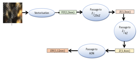
4.3 Original image preparation
Any original image must undergo modeling before entering the operating block to undergo a future encryption process and must go through the following steps:
4.3.1 Original image vectoring
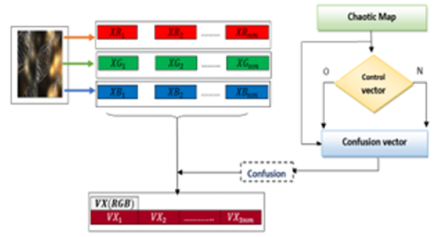
After extracting the three-color channels $(R G B)$ and converting them into vectors $(V r),(V g),(V b)$, each of dimension $(1, \mathrm{~nm})$, a concatenation operation controlled by the decision vector $\left(V B_1\right)$ is performed to generate a vector $(\mathrm{VX})=\left(\mathrm{VX}_1, \mathrm{VX}_2, \ldots, \mathrm{VX}_{\mathrm{n}_{\mathrm{nm}}}\right)$ of dimension $(1,3 \mathrm{~nm})$, as specified by Algorithm 3 below.
|
Algorithm 3: Original image vectoring algorithm |
|
For i=1 to nm if $V B_1(i)=0$ then $V X(3 i-2)=V r(i) \oplus V C_1(i)$ $V X(3 i-1)=V g(i) \oplus V C_2(i)$ $V X(3 i)=V b(i) \oplus V C_3(i)$ else $V X(3 i-2)=V r(i) \oplus V C_3(i)$ $V X(3 i-2)=V g(i) \oplus V C_1(i)$ $V X(3 i-2)=V b(i) \oplus V C_2(i)$ End if Next i |
This algorithm can be seen in Figure 1.
Figure 1. Original image vectoring diagram
The completion of this encryption step involves the computation of an initialization value closely linked to the original image and pseudo-random vectors.
4.3.2 Confusion / Diffusion process
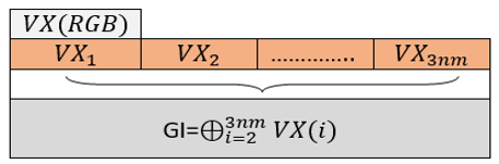
The initialization value (GI) involves the modification of the seed pixel's content, thus initiating the confusion/diffusion process. This value is calculated according to Algorithm 4 below.
|
Algorithm 4: Initialization value computation algorithm |
|
GI=0 For i=2 to 3 nm $G I=G I \bigoplus V X(i)$ Next i |
This algorithm can be represented by (Figure 2).
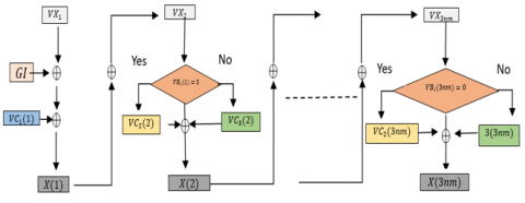
A first slight transformation of the vector (VX) into the vector (X) controlled by the vector (VB1) using diffusion and confusion operations, is given by the following algorithm:
|
Algorithm 5: Diffusion Phase algorithm |
|
// 1st pixel modification $X(1)=G I \oplus V X(1) \oplus V C_1(1)$ // next pixels modification For i=2 to 3 nm if VB1 (i)=0 then $X(i)=X(i-1) \oplus V X(i) \oplus V C_2(i)$ else $X(i)=X(i-1) \oplus V X(i) \oplus V C_3(i)$ End if Next i |
This algorithm can be illustrated by the Figure 3.
Figure 2. Initialization value computation diagram
Figure 3. Confusion and diffusion process diagram
To increase the temporal attack complexity of our system, we proceed with a second round acting at the DNA level and then at the RNA level through well-defined algebraic operations.
4.3.3 DNA coding
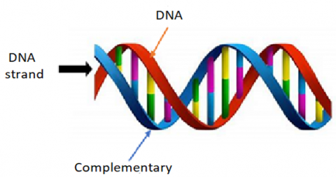
Definition. DNA, or deoxyribonucleic acid, is the molecule carrying the genetic code of an individual. This genetic information is present in all cells of the human body. The genetic code is represented by a sequence of four nucleotides: Adenine, Cytidine, Guanine, and Thymine, symbolized respectively by the letters A, C, G, and T as depicted in Table 1.
Table 1. Initial natural values of DNA nucleotides
|
Binary |
Chromosome DNA |
|
00 |
A |
|
01 |
C |
|
10 |
G |
|
11 |
T |
4.3.4 Pixels to nucleotides transformation
A pixel is converted into 4 nucleotides, each represented by two bits. This transition involves the following steps:
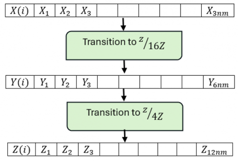
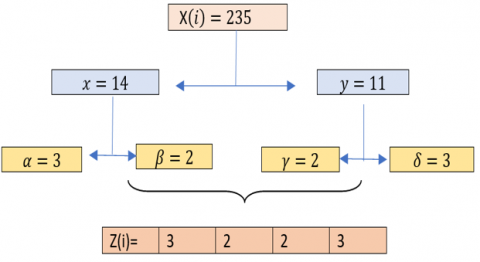
Transition to (Z⁄4Z). The output vector (X), with coefficients in (Z⁄256Z), is converted into a vector (Y) over (Z⁄16Z), and then into a vector (Z) over (Z⁄4Z) of size (1, 12 nm). This phase is illustrated by the diagram below (Figure 4):
This transition can be described by the following algorithm:
|
Algorithm 6: Transition to Z⁄4Z |
|
|
// Transition to DNA For i=1 to 3nm $x=E\left(\frac{X(i)}{16}\right)$ $y=\bmod (X(i), 16)$ $\alpha=E\left(\frac{x}{4}\right)$ β=mod(x,4) |
$\gamma=E\left(\frac{y}{4}\right)$ δ=mod(y, 4) Z(4i-3)=α Z(4i-2)=β Z(4i-1)=γ Z(4i)=δ Next i |
Figure 4. Transition to (Z⁄4Z)
Figure 5 give an example of such operation.
Figure 5. Transition table to (Z⁄4Z)
Transition to nucleotides. The transition from (Z⁄4Z) to nucleotides is a simple notation change, it can be defined by the following steps:
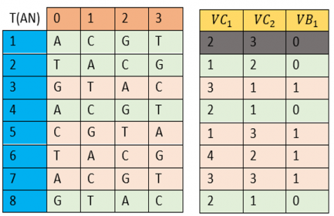
Transition from (Z⁄4Z) to DNA. The transition from (Z⁄4Z) to nucleotides is a simple notation change, whose pseudo-random selection of values for the components DNA of the table (AN) of size (8;4) is defined by:
The 1st row of the table ($A N$) is defined by the natural nucleotides’ 'A'=0, 'C'=1, 'G'=2, and 'T'=3.
·Any row of rank (i)$>$1 is obtained by shifting the previous row (i-1) by a pseudo-random step defined by the vector (VC1) or (VC2) depending on the values of the control vector (VB1).
Table construction (AN). The nucleotide table (AN) is generated by the following algorithm:
|
Algorithm 7: DNA table creation |
|
// First line AN(1,1)=”A”; AN(1,2)=”C” ; AN(1,3)=”G”; AN(1,4)=”T” // Next lines For i=2 to 8 For j=1 to 4 If $V B_1(i)=0$ then $A N(i, j)=A N\left(i-1,\left(j+V C_1(i) \% 4+1\right) \% 4+1\right)$ Else $A N(i, j)=A N\left(i-1,\left(j+V C_2(i) \% 4+1\right) \% 4+1\right)$ End if Next j, i |
An example of DNA table creation is depicted in Figure 6.
Figure 6. Example of DNA table creation
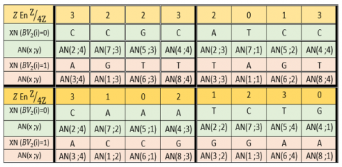
Nucleotides assignment. The vector (Z) will be transcribed into vector (XN), whose components are nucleotides read from the table (AN) based on the values of the control vector (VB2):
|
Algorithm 8: DNA vector construction |
|
// DNA vector For i=1 to 3nm $V B_2(i)=0$ then $\left.X N(4 i-3)=A N\left(V C_1(4 i-3) \% 8\right)+1, Z(i)+1\right)$ $\left.X N(4 i-2)=A N\left(V C_1(4 i-2) \% 8\right)+1, Z(i)+1\right)$ $\left.X N(4 i-1)=A N\left(V C_1(4 i-1) \% 8\right)+1, Z(i)+1\right)$ $\left.X N(4 i)=A N\left(V C_1(4 i) \% 8\right)+1, Z(i)+1\right)$ else $\left.X N(4 i-3)=A N\left(V C_2(4 i-3) \% 8\right)+1, Z(i)+1\right)$ $\left.X N(4 i-2)=A N\left(V C_2(4 i-2) \% 8\right)+1, Z(i)+1\right)$ $\left.X N(4 i-1)=A N\left(V C_2(4 i-1) \% 8\right)+1, Z(i)+1\right)$ $\left.X N(4 i)=A N\left(V C_2(4 i) \% 8\right)+1, Z(i)+1\right)$ End if Next i |
Note:
A simple perturbation to the secret key of the system results in the generation of a new DNA table (AN), and consequently, a new vector (XN). This table may have a pseudo-random dimension computed from the used chaotic maps.
The transition from the initial image to DNA notation is described in the following Figure 7.
Example:
Nucleotides Complementary. Each nucleotide has a unique complementary counterpart in RNA duplication. Naturally, the complements of nucleotides are defined in the following table:
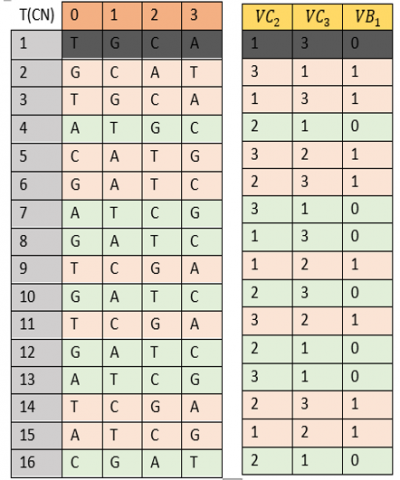
In our work, the complement of a nucleotide will be determined by a pseudo-random table (CN) of size (16;4) generated through the following steps:
·1st line is constructed from natural complementariness.
·The line j>1 is the shifting of the line j-1 of rank VC2 (j) or VC3 (j) across the VB1 (j) control value.
The construction of the nucleotide complement (CN) table is described by the algorithm below.
|
Algorithm 9: Construction of the nucleotide complement (CN) table |
|
// First line CN(1,1)=”T” CN(1,2)=”G” CN(1,3)=”C” CN(1,4)=”A” // next Lines For j=2 to 8 For k=1 to 4 If $V B_2(j)=0$ then $\mathrm{CN}(\mathrm{j}, \mathrm{k})=\mathrm{CN}\left(\mathrm{j}-1,\left(\mathrm{k}+V C_3(j) \% 4+1\right) \% 4+1\right)$ Else $\mathrm{CN}(\mathrm{j}, \mathrm{k})=\mathrm{CN}\left(\mathrm{j}-1,\left(\mathrm{k}+V C_2(j) \% 4+1\right) \% 4+1\right)$ End if Next k,j |
This algorithm can be represented by Figure 8 below.
Figure 7. Transition to DNA
Figure 8. Construction of table (CN)
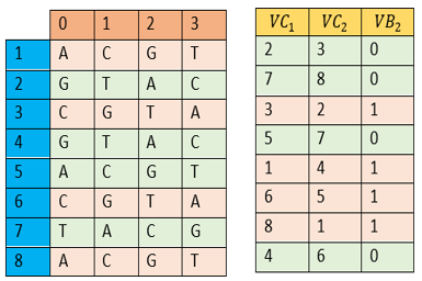
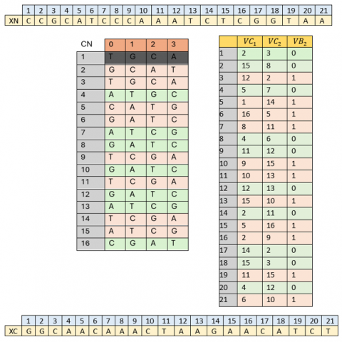
The vector (XC) of complementary nucleotides to vector (XN) is determined by the following algorithm:
|
Algorithm 10: construction of Vector (XC) |
|
For i=1 to 12nm If XN(i)=”A” then Col=0 else If $X N(i)=" C "$ then Col=1 else If XN(i)=”G” then Col=2 else If XN(i)=”T” then Col=3 End if if VB2 (i)=0 then $\left.X C(i)=C N\left(V C_1(i) \% 16\right)+1 ; C o l\right)$ else $\left.X C(i)=C N\left(V C_2(i) \% 16\right)+1 ; C o l\right)$ End if Next i |
The complementary strand forms the double helix of the DNA strand (Figure 9).
Figure 10 depict an example of vector (XC) transformation to vector (XN).
We observe that the location and values of the complements are closely related to the table (CN) and are taken in a pseudorandom manner.
DNA pseudorandom vector construction. We observe that the location and values of the complements are closely linked to the table (CN) and taken in a pseudo-random manner. A pseudo-random vector (BD) with DNA coefficients is constructed to introduce confusion with vectors (XN) and (XC) under the control of (VB3). This construction is determined by the algorithm below:
|
Algorithm 11: DNA pseudorandom vector generation |
|
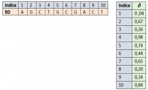
For i=1 to 12nm if ϑ(i)<0,25 then BD(i)="A" else if ϑ(i)<0,5 then BD(i)="C" else if ϑ(i)<0,75 then BD(i)="G" else BD(i)="T" End if Next i |
Figure 11 depict an example of Algorithm 10 above.
Figure 9. (XN) pseudorandom vector generation DNA
Figure 10. Example of vector (XC) conversion to vector (XN)
Figure 11. Example of DNA pseudorandom vector generation
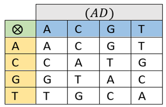
Genetic algebraic operator. An algebraic operator (⨂) between DNA values will be established under the control of the following table (AD). This operator is depicted in (Figure 12) below.
Figure 12. Genetic operator
The algebraic operator $(\otimes)$ employed to link two nucleotides is a reversible, commutative operator that provides a group structure to facilitate transformations on DNA. Figure 13 give an example of such operation.
Figure 13. Algebraic operator $(\otimes)$ application example
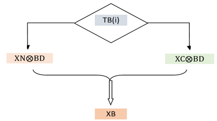
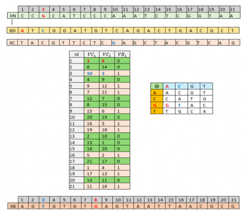
DNA genetic crossover. The vectors (XN) and (XC) undergo genetic crossover with the vector (BD) to generate a new vector (XB) with DNA components, under the control of the table (TB) of size (12 nm; 3).
Construction crossover of table (TB):
·The first column obtained by sorting in ascending order the 12nm values of (VC1) vector;
·The second column obtained by sorting in ascending order the 12nm values of (VC2) vector;
·The third column is the (VB1) vector.
Description of the role of the table (TB):
·The 1st column indicates the index of the vector (XN) or the vector (XC). Crossed with the following vector (BD);
·The second column gives the index of the position in the vector (XB);
·The third column indicates the choice of the vector (XN) or (XC) crossed with the vector (BD) through a genetic crossover table (AD).
·This genetic crossover at the DNA level is described by the following algorithm:
|
Algorithm 12: Genetic DNA crossover |
|
For i to 4nm If TB(i;3)=0 then $X B(T B(i ; 2))=X N(T B(i ; 1) \otimes B D(i))$ Else $X B(T B(i ; 2))=X C(T B(i ; 1) \otimes B D(i))$ Next i |
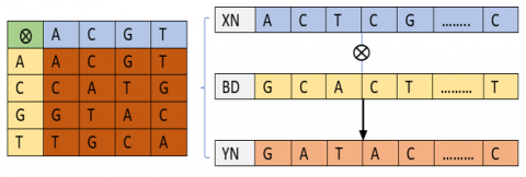
This passage is defined by the following diagram (Figure 14).
An example of such transformation is depicted in Figure 15.
Figure 14. DNA crossover operation
Figure 15. Genetic DNA crossover transformation
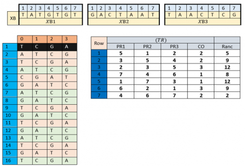
Transition to RNA. RNA is the concatenation of three nucleotides read from a gene for the formation of a protein. For this, the vector (XB) is subdivided into three sub-vectors (XB₁), (XB₂), and (XB₃) each of size (1; 4 nm). The transition from DNA to RNA requires the construction of the table (TR) of size (4 nm; 5) defined by the following process:
·The first column is the arrangement (PR1), which is obtained by roughly sorting the first 4 nm values of (VC1) in ascending order;
·The second column is the arrangement (PR2), which is obtained by roughly sorting the first 4nm values of (VC2) in ascending order;
·The third column is the arrangement (PR3), which is obtained by roughly sorting the first 4 nm values of (VC3) in ascending order;
·The fourth column is the 4 nm vector values (CO);
·The fifth column is the vector (VE).
Construction of (TR) table. These table construction steps (TR) are defined by:
|
Algorithm 13: Construction of the (TR) transition table |
|
For i =1 to 4nm $T R(i, 1)=P R 1(i)$ $T R(i, 2)=P R 2(i)$ $T R(i, 3)=P R 3(i)$ $T R(i, 4)=C O(i)$ $T R(i, 5)=V E(i)$ Next i |
Description of the table (EN):
·The first column gives the index of nucleotides in the sub vector (XB1);
·The 2nd column gives the index of nucleotides in the sub vector (XB2);
·The 3rd column gives the index of nucleotides in the sub vector (XB3);
·The 4th column gives the index of the nucleotides that should be transcribed in complementary;
·The 5th column gives the row in the table (CN) for selecting the nucleotide value.
Figure 16 depict an example of (TR) table transition.
Figure 16. Transition table (TR) example
The conversion of nucleotides into RNA is given by the following algorithm:
|
Algorithm 14: Construction of the (XR) vector |
|
For i=1 to 4nm x=XB1(TR(i,1)) y=XB2(TR(i,2)) z=XB3(TR(i,3)) if co(i)=1 then x=compl(x) if co(i)=2 then y=compl(y) if co(i)=3 then z=compl(z) XR(i)=x&y&z Next i |
Figure 17 depict an example of transition from nucleotides to codons.
Figure 17. Transition from nucleotides to codons example
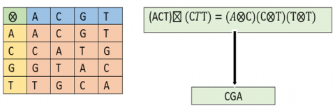
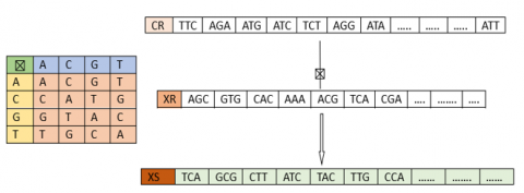
Algebraic operation $(\boxtimes)$ on RNA. Using the operator table $(A D)$, it is possible to combine two RNA through the following genetic operation: $(x y z) \boxtimes(u v w)=(x \otimes u)(y \otimes v)(z \otimes w)$.
On the other hand, the algebraic operator $(\boxtimes)$ used to link two codons is a reversible, commutative operator applied to RNA, dependent on $(\otimes)$. However, it is noteworthy that in the case of RNA, only one nucleotide at a time undergoes complementarity under the control of the control vector (CR).
An example of algebraic operator ( $\boxtimes)$ application is depicted in Figure 18.
Figure 18. example of algebraic operator $(\boxtimes)$ application
We notice that the algebraic operation defined on the RNA is not commutative, which increases the complexity of attacks on our cryptographic system.
RNA crossover.
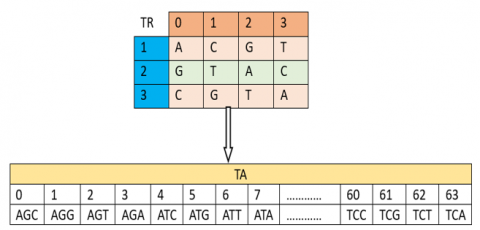
Construction of the reference RNA table
In a first step, a reference RNA table (TA) of size (2; 64) is constructed by the following process:
The 1st row is given by the following algorithm:
|
Algorithm 15.1: Construction of the (TA) table |
|
For i=1 to 64 TA(1; i)=i-1 Next i |
The second line includes codons whose numerical value is associated with the first line generated by the algorithm below:
|
Algorithm 15.2: Construction of the (TA) table |
|
For i=1 to 4 For j=1 to 4 For k=1 to 4 TA(2;i)=TR(1;i)&TR(2;j)&TR(3;k) Next k, j, i |
This algorithm can be explained by an example depicted in Figure 19 below.
Figure 19. Construction of the (TA) table example
The construction of the reference table (TA) is closely related to the nucleotide table (TR).
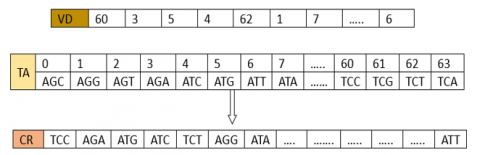
Generation of the pseudo-random vector (CR) with coefficient (RNA)
A vector (CR) with pseudo-random component RNA taking values from the reference table (TA) is constructed by the following process:
|
Algorithm 16: Construction of the (CR) vector |
|
For i=1 to 4nm CR(i)=TA(2; VD(i)) Next i |
Construction of the (CR) vector is explained by an example depicted in Figure 20 below.
Figure 20. Construction of the (CR) vector
The vector (XS) obtained through genetic crossover between the chaotic vector (CR) and the vector (XR) at the RNA level is given by the following algorithm:
|
Algorithm 17: Construction of the (XS) vector |
|
For i=1 to 4nm $\mathrm{XS}(i)=\mathrm{XR}(\mathrm{i}) \boxtimes C R(\mathrm{i})$ Next i |
The vector (XS) represents the RNA-coefficient encrypted image using our approach. Figure 21 represents an example of the (XS) vector construction.
Figure 21. Construction of the (XS) vector example
Example:
Reconstruction of the encrypted image
The reconstruction of the encrypted image from the vector (XS) with RNA coefficient requires going through the following steps:
·Transition to DNA
The transition from RNA to DNA notation is ensured by the reference table (RT).
Example:
The transition from vector (XS) to vector (XD) in DNA is determined by the following algorithm:
·Transition to (Z⁄4Z)
We assume: ‘A’=0, ‘C’=1, ‘G’=2 et ‘T’=3
The vector (XD) will be converted to $(X T)$ with a coefficient of (Z⁄4Z):
|
Algorithm 18: Transition to (Z⁄4Z) |
|
|
For i=1 to 12nm if XS(i)="A" then XT(i)=0 Else if XS(i)="C" then XT(i)=1 else |
if XS(i)="G" then XT(i)=2 else if XS(i)="T" then XT(i)=3 End if Next i |
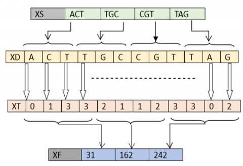
The vector (XT) will be converted to degree level to (XF) by the following process:
|
Algorithm 19: Transition to (Z⁄256Z) |
|
For i=1 to 3nm $\begin{aligned} & X F(i)=X T(4 i-3) * 4^3+X T(4 i-2) * 4^2+X T(4 i- \\ & 1) * 4^1+X T(4 i) * 4^0\end{aligned}$ Next i |
An example of transition to (Z⁄256Z) is depicted in Figure 22 below.
Figure 22. Transition to (Z⁄256Z) example
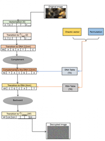
4.4 Decryption of the encrypted image
Our algorithm is characterized by a symmetric encryption system, involving the use of an identical key during the decryption process and the same encryption parameters. As our approach employs diffusion functions, the decryption procedure must start with the last encrypted block by applying the inverse functions of the corresponding encryption functions. This decryption process involves the following sequences:
·Encrypted image loading;
·Encryption key generation;
·Encoding of the encrypted image in RNA phase;
·Encoding of the encrypted image in DNA phase;
·Reverse genetic crossover;
·Transition to (Z⁄256Z);
·Confusion section;
·Construction of the original image.
These steps are illustrated by the diagram (Figure 23).
Figure 23. Decryption scheme
All experiments were conducted using the Python programming language on Windows 10, with a hardware environment consisting of a laptop with an i5 processor, 8 GB of RAM, and a hard drive with a capacity of 256 GB.
5.1 Analysis of brute force attack
Our recent algorithm underwent an evaluation using a set of randomly selected reference images, and the results of successive simulations were recorded.
5.2 Key space analysis
The algorithm we have designed exploits two chaotic maps generated from four parameters, each coded on 32 bits.
Hence, the overall secret key space is 128 bits, which is significantly larger than 100 bits, ensuring that our approach is safe from any brute-force attacks.
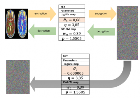
5.3 Key sensitivity
Our system harnesses two chaotic maps widely embraced in the field of cryptography due to their extreme sensitivity to initial conditions. This characteristic imparts a high sensitivity to our encryption key. This property can be visualized in the following diagram (Figure 24):
Figure 24. Key sensitivity
We confirm that any slight disturbance to one of the parameters of the secret key results in a poor encrypted image.
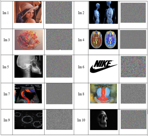
5.4 Visual aspect
It is crucial to note that the encrypted image shows visual distinctions compared to the original image, as demonstrated in Figure 25. Furthermore, it is important to emphasize that all histograms of the images encrypted by our algorithm exhibit a uniform distribution, thus confirming effective protection against any attempts of statistical attacks.
Visually, an encrypted image is completely different from a clear image, and it bears no resemblance to a highlight.
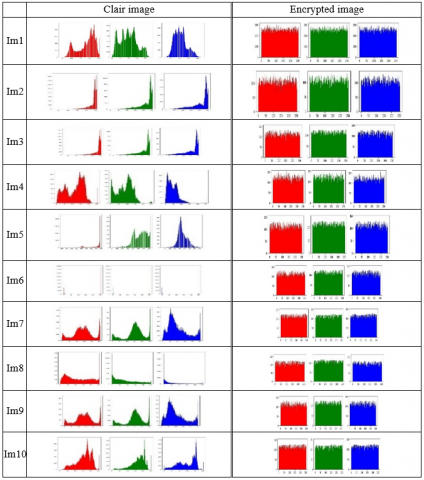
5.5 Analysis of histograms
The statistical distribution of individual pixels is depicted in the image's histogram. Due to the multitude of information contained in the raw image, it is crucial to note that the encrypted image manifests visual distinctions compared to the original image, as demonstrated in Figure 26. Furthermore, it should be emphasized that all histograms of images encrypted by our algorithm exhibit a uniform distribution, thus corroborating effective protection against any attempts of statistical attacks.
Figure 25. Visual aspect
Figure 26. (RGB) channels histograms of encrypted images
Table 2. Comparison of histogram variance
|
Image |
Im1 |
Im2 |
Im3 |
Im4 |
Im5 |
Im6 |
||
|
Original |
R |
123072.50 |
620306.75 |
289630.65 |
992034.12 |
129825.53 |
129765.98 |
|
|
G |
87100.83 |
860899.31 |
337863.062 |
1330180.12 |
57011.605 |
349251.718 |
||
|
B |
33522.73 |
790776.56 |
210359.812 |
768126.75 |
81373.710 |
537500.062 |
||
|
Encrypted |
Proposed |
R |
218.99 |
262.241 |
275.069 |
1136.54 |
250.867 |
214.759 |
|
G |
231.02 |
233.21 |
242.961 |
1109.79 |
214.998 |
258.798 |
||
|
B |
220.991 |
254.804 |
238.089 |
1059.99 |
257.959 |
237.997 |
||
|
[28] |
R |
219.513 |
262.265 |
275.095 |
1136.56 |
250.877 |
214.782 |
|
|
G |
231.052 |
233.211 |
243.858 |
1119.74 |
215.093 |
259.715 |
||
|
B |
221.119 |
255.813 |
238.196 |
1060.54 |
258.754 |
238.384 |
||
|
[29] |
R |
247.78 |
280.64 |
284.35 |
1070.2 |
282.81 |
232.98 |
|
|
G |
279.62 |
280.46 |
247.37 |
1231.2 |
254.87 |
279.61 |
||
|
B |
265.71 |
230.42 |
260.76 |
941.65 |
225.79 |
245.61 |
||
5.6 Variances of histograms
In a similar manner, by determining the histogram variance given in Eq. (3), we evaluated the coherence of encrypted images. Lower variance in an encrypted image indicates increased uniformity and a higher level of security for the contemplated image encryption algorithm [26, 27].
$H_{V a r}(X)=\frac{1}{3 n m} \sum_{p=1}^{255}\left|\left(x o_p-x c_p\right)\right|$ (3)
where, xop Number of the clear pixel of value p, xcp Encrypted pixel count of value p.
Table 2 displays the standard deviations associated with specific test images. The data in the table reveals that clear images exhibited disproportionately high standard deviations, whereas encrypted images demonstrated notably low values. To illustrate, the average standard deviation for the encrypted image (Im1) was 223.667, significantly lower than the corresponding clear image with a standard deviation of 81,232.023. Additionally, the comparison presented suggests that, for most test images, the histogram standard deviations of images encrypted using the proposed algorithm were consistently lower than those of Alawida et al. [28] and Zhang et al. [29]. Based on this comparison, we can assert that our proposed algorithm has the ability to enhance the security of the encryption algorithm.
5.7 Entropy analysis
The entropy of an image of size (n, m) is given by Eq. (4).
$S H(M C)=\frac{-1}{3 n m} \sum_{i=1}^{3 n m} p(i) \cdot \log _2(p(i))$ (4)
where, $p(i)$ is the probability of the occurrence of level (i) in the original image. Thus, as entropy approaches this reference, the quality of the random distribution of pixels in the image improves. Higher entropy ensures a significant reduction in the amount of recoverable information from the specific encrypted image. The table titled Table 3 displays the entropy values for our test images in comparison to existing image encryption algorithms. The table reveals that the values, with $\mathrm{SH} \geqslant 7.996$, are comparable to the study of Gera and Agrawal [30] and surpass those of Alawida et al. [28].
5.8 Correlation analysis
The correlation of the image of size (n, m) is given by Eq. (5).
$\operatorname{corr}=\frac{\operatorname{cov}(x, y)}{\sqrt{\operatorname{var}(x)} \cdot \sqrt{\operatorname{var}(y)}}$ (5)
Table 4 presents the correlations between pixels in the image (Im1). A comparative analysis with previous algorithms reveals a lower correlation between adjacent pixels in our encrypted image compared to the studies of Gera and Agrawal [30], Zhang et al. [31], and Soltani et al. [32], although this correlation remains comparable to that observed in the studies of Alawida et al. [28], Sun et al. [33], Tahbaz et al. [34], and Jarjar et al. [35]. Table 3 displays correlation coefficients for pixels derived from images in the SIPI database and additional test images. The table reveals a notably high correlation within clear images, approaching nearly “1” for each channel. Conversely, images encrypted by our proposed algorithm exhibit significantly lower correlation based on the data presented in the table. These observations confirm the satisfactory level of security provided by our algorithm. These findings emphasize a notable reduction in correlation within the encrypted image, indicating that potential attackers are unable to extract information through this approach.
The correlation measures for the images evaluated using our encryption system consistently approach zero. This feature serves as a safeguard against statistical attacks, as indicated in Table 5.
Table 3. Entropy examination of encrypted images in contrast to alternative methods
|
Algorithm |
Images |
Ciphered |
||
|
R |
G |
B |
||
|
Proposée |
Im1 |
7.9973 |
7.9974 |
7.9971 |
|
Im2 |
7.9994 |
7.9994 |
7.9995 |
|
|
Im3 |
7.9994 |
7.9992 |
7.9994 |
|
|
Im4 |
7.9975 |
7.9971 |
7.9974 |
|
|
Im5 |
7.9994 |
7.9995 |
7.9993 |
|
|
[30] |
Im1 |
7.9972 |
7.9973 |
7.9970 |
|
Im2 |
7.9993 |
7.9994 |
7.9994 |
|
|
Im3 |
7.9993 |
7.9992 |
7.9993 |
|
|
Im4 |
7.9974 |
7.9970 |
7.9974 |
|
|
Im5 |
7.9993 |
7.9994 |
7.9993 |
|
|
[28] |
Im1 |
7.9974 |
7.9974 |
7.9971 |
|
Im2 |
7.9993 |
7.9994 |
7.9992 |
|
|
Im3 |
7.9993 |
7.9992 |
7.9993 |
|
|
Im4 |
7.9972 |
7.9971 |
7.9966 |
|
|
Im5 |
7.9992 |
7.9994 |
7.9994 |
|
Table 4. Correlation among the pixels in the encrypted 'Im1' image
|
Algorithm |
Horizontal |
Vertical |
Diagonal |
|
Proposed |
-0.002733667 |
0.00352 |
-0.002469667 |
|
[28] |
-0.0042707 |
-0.0032498 |
-0.0020192 |
|
[30] |
-0.0029883 |
0.0091357 |
-0.0067375 |
|
[31] |
-0.0098 |
-0.0050 |
-0.0013 |
|
[32] |
0.0080 |
0.0098 |
-0.0058 |
|
[33] |
-0.0023 |
0.0019 |
-0.0034 |
|
[34] |
0.0020 |
-0.0007 |
-0.0014 |
|
[35] |
-0.0237 |
-0.0178 |
-0.0284 |
Table 5. Correlation between pixels of the selected images from the database (SIP)
|
Images |
Original image |
Encrypted image |
||||||
|
H |
V |
D |
H |
V |
D |
|||
|
Im1 |
R |
0.9558 |
0.9648 |
0.9325 |
-0.003771 |
0.008149 |
-0.00132 |
|
|
G |
0.93556 |
0.95756 |
0.91902 |
-0.002981 |
0.009127 |
-0.006732 |
||
|
B |
0.90773 |
0.9393 |
0.8913 |
-0.001449 |
-0.006716 |
0.000643 |
||
|
Im2 |
R |
0.98385 |
0.96944 |
0.98629 |
-0.0013662 |
-0.0018756 |
-0.0054082 |
|
|
G |
0.97883 |
0.98511 |
0.96537 |
-0.0010662 |
0.0015054 |
0.0023428 |
||
|
B |
0.99153 |
0.98348 |
0.98724 |
0.0048931 |
-0.0057105 |
-0.0011768 |
||
|
Im3 |
R |
0.95175 |
0.96552 |
0.93161 |
0.0051302 |
-0.0007677 |
-0.0049534 |
|
|
G |
0.95215 |
0.96436 |
0.93066 |
0.0078786 |
-0.0007949 |
0.0002736 |
||
|
B |
0.95542 |
0.97086 |
0.94265 |
0.000070 |
0.0109689 |
-0.0010586 |
||
|
Im4 |
R |
0.98681 |
0.99219 |
0.97287 |
-0.0043816 |
-0.0165139 |
0.0066847 |
|
|
G |
0.98851 |
0.99103 |
0.97352 |
0.0023923 |
0.0017955 |
-0.0034511 |
||
|
B |
0.98675 |
0.99049 |
0.97189 |
0.0087519 |
0.0057946 |
-0.0030269 |
||
|
Im5 |
R |
0.95839 |
0.95430 |
0.91674 |
-0.0014431 |
-0.0019301 |
0.0075854 |
|
|
G |
0.89596 |
0.95015 |
0.87160 |
-0.0012697 |
0.0075575 |
-0.001531 |
||
|
B |
0.91304 |
0.93012 |
0.86383 |
-0.0014109 |
0.0010211 |
-0.0038232 |
||
|
Im6 |
R |
0.97886 |
0.98012 |
0.96108 |
0.0012429 |
-0.0032612 |
0.0007536 |
|
|
G |
0.97749 |
0.97952 |
0.95947 |
-0.0007566 |
-0.0024509 |
0.0044757 |
||
|
B |
0.97224 |
0.97091 |
0.94729 |
-0.0010254 |
-0.0049974 |
0.0015236 |
||
|
Im7 |
R |
0.98679 |
0.98515 |
0.97406 |
-0.0044956 |
-0.0014317 |
0.0047762 |
|
|
G |
0.98083 |
0.98077 |
0.96404 |
-0.0057874 |
-0.0009189 |
-0.0066636 |
||
|
B |
0.95393 |
0.94939 |
0.90846 |
-0.0040614 |
0.0012302 |
-0.0055081 |
||
|
Im8 |
R |
0.97833 |
0.97815 |
0.96277 |
-0.0061589 |
0.0021684 |
0.002564 |
|
|
G |
0.99106 |
0.99427 |
0.97853 |
-0.0021031 |
0.0011387 |
0.0099093 |
||
|
B |
0.99370 |
0.99471 |
0.98813 |
-0.0036710 |
-0.0012494 |
0.0046701 |
||
To assess how well the algorithm performs under differential attacks, metrics such as the Number of Pixel Changes Rate (NPCR), Unified Average Change Intensity (UACI), and the avalanche effect are employed.
6.1 NPCR constant
The NPCR is determined by Eq. (6).
$N P C R=\left(\frac{1}{3 n m} \sum_{i, j=1}^{n m} D(i, j)\right) \cdot 100$ (6)
where,
$D(i, j)=\left\{\begin{array}{lll}1 & \text { if } & C_1(i, j) \neq C_2(i, j) \\ 0 & \text { if } & C_1(i, j)=C_2(i, j)\end{array}\right.$
6.2 UACI constant
The analysis of the mathematical constant $U A C I$ of the image is given by the Eq. (7).
$U A C I=\left(\frac{1}{255 n m} \sum_{i, j=1}^{n m} A B S\left(C_1(i, j)-C_2(i, j)\right)\right) \cdot 100$ (7)
The data in Table 6 presents the measures of NPCR and UACI for two images (Im1, Im2), showing that NPCR ≥ 99.6 and UACI≥33.4. These values clearly indicate that the performance of the NPCR of the proposed encryption algorithm was comparable to that of Alawida et al. [28] and superior to that of Manzoor et al. [36], Alawida et al. [37], Teseleanu [38], Jarjar et al. [39], Ye and Huang [40], and Chen et al. [41], while the UACI value was comparable to those of others.
6.3 Robustness against occlusion attacks
In the field of image processing, the parameters of Mean Squared Error (MSE) and Peak Signal-to-Noise Ratio (PSNR) are frequently used to assess the quality of encryption. These metrics are the most commonly employed criteria for evaluating the quality of two images within a cryptographic system. PSNR measures the similarity between two images and is the complement of MSE. The Mean Squared Error (MSE) for the original, decrypted, and encrypted images can be computed using the following formula (8):
$M S E=\frac{1}{(n m)^2} \sum_{i, j=1}^{n m}|\operatorname{Imo}(i, j)-\operatorname{Imc}(i, j)|^2$ (8)
In the context of image processing) "Imo" and "Imc" respectively represent the original and encrypted images. MSE corresponds to the mean squared error. (n) denotes the number of rows in the original image, and (m) represents the number of columns in the image. PSNR is evaluated in decibels and is inversely proportional to the mean squared error. It is determined by Eq. (9).
$P S N R=10 * \log _{10}\left(\frac{\left(2^L-1\right)^2}{M S E}\right)(d B)$ (9)
where, L=8 represents the bit depth of the specific image.
A greater PSNR signifies reduced differences between the original and decrypted images as represented in Table 7. When the original and encrypted images are identical, their PSNR becomes infinite.
Table 6. Comparison of (NPCR) and (UACI)
|
Algorithm |
Im1 |
Im2 |
||
|
NPCR |
UACI |
NPCR |
UACI |
|
|
Proposed |
99.68 |
33.49 |
99.67 |
33.48 |
|
[28] |
99.68 |
33.46 |
99.67 |
33.48 |
|
[30] |
99.60 |
33.49 |
99.61 |
33.46 |
|
[36] |
99.66 |
33.44 |
99.63 |
33.47 |
|
[37] |
99.61 |
33.46 |
99.60 |
33.49 |
|
[38] |
99.59 |
33.46 |
- |
- |
|
[39] |
99.60 |
33.44 |
- |
- |
|
[40] |
99.62 |
33.65 |
- |
- |
|
[41] |
99.61 |
33.47 |
- |
- |
Table 7. (PSNR) (dB) between the original image, the encrypted image, and the decrypted image
|
Algorithm |
PSNR type |
Lena |
Baboon |
Panda |
Vegetables |
|
Proposed |
Original to decrypted |
$\infty$ |
$\infty$ |
$\infty$ |
$\infty$ |
|
Original to decrypted |
8.1212 |
8.7811 |
8.1748 |
6.8800 |
|
|
[28] |
Original to decrypted |
$\infty$ |
$\infty$ |
$\infty$ |
$\infty$ |
|
|
Original to decrypted |
8.1102 |
8.7776 |
8.1648 |
6.8760 |
|
[37] |
Original to decrypted |
8.1300 |
7.8569 |
7.7410 |
7.4395 |
|
[38] |
Original to decrypted |
8.3655 |
8.8532 |
- |
- |
|
[39] |
Original to decrypted |
8.2522 |
8.8223 |
- |
- |
|
[40] |
Original to decrypted |
$\infty$ |
$\infty$ |
- |
- |
|
|
Original to decrypted |
7.0257 |
7.1515 |
- |
- |
Cryptography has embraced chaos theory, leveraging the pronounced sensitivity of chaotic systems to their starting states. Our approach capitalizes on this attribute through the utilization of RNA genetic crossover. The incorporation of genetic crossover, guided by a pseudo-random table, imparts substantial value and intricacy to a novel encryption system. This is substantiated by the observed values of statistical and differential constants in simulations across a diverse set of images randomly selected from multiple databases.
I would like to express my gratitude to all the authors who have contributed, directly or indirectly, to the completion of this article. I would like to emphasize that our research group is not supported by any public or private organization.
|
RNA |
Ribonucleic Acid |
|
DNA |
Deoxyribonucleic Acid |
|
GA |
Genetic Algorithm |
|
Greek symbols |
|
|
η |
Control parameter chaotic map |
|
ϑ0 |
Initial condition chaotic map |
|
t0 |
Initial condition chaotic PWLCM |
|
h |
Control parameter chaotic PWLCM |
[1] Sharma, S., Ramkumar, K.R., Kaur, A., Hasija, T., Mittal, S., Singh, B. (2023). Post-quantum cryptography: A solution to the challenges of classical encryption algorithms. Modern Electronics Devices and Communication Systems: Select Proceedings of MEDCOM 2021, 23-38. https://doi.org/10.1007/978-981-19-6383-4_3
[2] Haq, I., Mazhar, T., Malik, M.A., Kamal, M.M., Ullah, I., Kim, T., Hamdi, M., Hamam, H. (2022). Lung nodules localization and report analysis from computerized tomography (CT) scan using a novel machine learning approach. Applied Sciences, 12(24): 12614. https://doi.org/10.3390/app122412614
[3] Elsaid, S.A., Alotaibi, E.R., Alsaleh, S. (2023). A robust hybrid cryptosystem based on DNA and Hyperchaotic for images encryption. Multimedia Tools and Applications, 82(2): 1995-2019. https://doi.org/10.1007/s11042-022-12641-5
[4] Gao, X., Mou, J., Banerjee, S., Cao, Y., Xiong, L., Chen, X. (2022). An effective multiple-image encryption algorithm based on 3D cube and hyperchaotic map. Journal of King Saud University-Computer and Information Sciences, 34(4): 1535-1551. https://doi.org/10.1016/j.jksuci.2022.01.017
[5] Zhu, L., Xie, Y., Zhou, Y., Fan, Q., Zhang, C., Liu, X. (2023). Enabling efficient and secure health data sharing for Healthcare IoT systems. Future Generation Computer Systems, 149: 304-316. https://doi.org/10.1016/j.future.2023.07.031
[6] Balasamy, K., Shamia, D. (2023). Feature extraction-based medical image watermarking using fuzzy-based median filter. IETE Journal of Research, 69(1): 83-91. https://doi.org/10.1080/03772063.2021.1893231
[7] Kumar, D., Sudha, V.K., Ranjithkumar, R. (2023). A one-round medical image encryption algorithm based on a combined chaotic key generator. Medical & Biological Engineering & Computing, 61(1): 205-227. https://doi.org/10.1007/s11517-022-02703-z
[8] Guan, M., Yang, X., Hu, W. (2019). Chaotic image encryption algorithm using frequency-domain DNA encoding. IET Image Processing, 13(9): 1535-1539. https://doi.org/10.1049/iet-ipr.2019.0051
[9] Mahmud, M., Lee, M., Choi, J.Y. (2020). Evolutionary-based image encryption using RNA codons truth table. Optics & Laser Technology, 121: 105818. https://doi.org/10.1016/j.optlastec.2019.105818
[10] Abbasi, A.A., Mazinani, M., Hosseini, R. (2020). Chaotic evolutionary-based image encryption using RNA codons and amino acid truth table. Optics & Laser Technology, 132: 106465. https://doi.org/10.1016/j.optlastec.2020.106465
[11] Yadollahi, M., Enayatifar, R., Nematzadeh, H., Lee, M., Choi, J.Y. (2020). A novel image security technique based on nucleic acid concepts. Journal of Information Security and Applications, 53: 102505. https://doi.org/10.1016/j.jisa.2020.102505
[12] Wang, X., Guan, N. (2020). A novel chaotic image encryption algorithm based on extended Zigzag confusion and RNA operation. Optics & Laser Technology, 131: 106366. https://doi.org/10.1016/j.optlastec.2020.106366
[13] Kanwal, S., Inam, S., Othman, M.T.B., Waqar, A., Ibrahim, M., Nawaz, F., Nawaz, Z., Hamam, H. (2022). An effective color image encryption based on Henon map, tent chaotic map, and orthogonal matrices. Sensors, 22(12): 4359. https://doi.org/10.3390/s22124359
[14] Wang, Y., Liu, S., Khan, A. (2023). On fractional coupled logistic maps: Chaos analysis and fractal control. Nonlinear Dynamics, 111(6): 5889-5904. https://doi.org/10.1007/s11071-022-08141-8
[15] Fan, S., Chen, K., Tian, J. (2023). A novel image encryption algorithm based on coupled map lattices model. Multimedia Tools and Applications, 83: 11557-11572. https://doi.org/10.1007/s11042-023-15964-z
[16] Daoui, A., Karmouni, H., Sayyouri, M., Qjidaa, H. (2022). Robust image encryption and zero-watermarking scheme using SCA and modified logistic map. Expert Systems with Applications, 190: 116193. https://doi.org/10.1016/j.eswa.2021.116193
[17] Yang, Y., Wang, L., Duan, S., Luo, L. (2021). Dynamical analysis and image encryption application of a novel memristive hyperchaotic system. Optics & Laser Technology, 133: 106553. https://doi.org/10.1016/j.optlastec.2020.106553
[18] Liu, Z., Wu, C., Wang, J., Hu, Y. (2019). A color image encryption using dynamic DNA and 4-D memristive hyper-chaos. IEEE Access, 7: 78367-78378. https://doi.org/10.1109/ACCESS.2019.2922376
[19] Kumar, V., Girdhar, A. (2021). A 2D logistic map and Lorenz-Rossler chaotic system based RGB image encryption approach. Multimedia Tools and Applications, 80: 3749-3773. https://doi.org/10.1007/s11042-020-09854-x
[20] Zhang, G., Ding, W., Li, L. (2020). Image encryption algorithm based on tent delay-sine cascade with logistic map. Symmetry, 12(3): 355. https://doi.org/10.3390/sym12030355
[21] Rakheja, P., Vig, R., Singh, P. (2020). Double image encryption using 3D Lorenz chaotic system, 2D non-separable linear canonical transform and QR decomposition. Optical and Quantum Electronics, 52: 1-21. https://doi.org/10.1007/s11082-020-2219-8
[22] Liang, Z., Qin, Q., Zhou, C., Xu, S. (2023). Color image encryption algorithm based on four-dimensional multi-stable hyper chaotic system and DNA strand displacement. Journal of Electrical Engineering & Technology, 18(1): 539-559. https://doi.org/10.1007/s42835-022-01157-5
[23] Zhu, Y., Wang, C., Sun, J., Yu, F. (2023). A chaotic image encryption method based on the artificial fish swarms algorithm and the DNA coding. Mathematics, 11(3): 767. https://doi.org/10.3390/math11030767
[24] Zhu, S., Deng, X., Zhang, W., Zhu, C. (2023). Image encryption scheme based on newly designed chaotic map and parallel DNA coding. Mathematics, 11(1): 231. https://doi.org/10.3390/math11010231
[25] Yao, X., Xie, R., Zan, X., Su, Y., Xu, P., Liu, W. (2023). A novel image encryption scheme for DNA storage systems based on DNA hybridization and gene mutation. Interdisciplinary Sciences: Computational Life Sciences, 15: 419-432. https://doi.org/10.1007/s12539-023-00565-z
[26] Qobbi, Y., Jarjar, A., Essaid, M., Benazzi, A. (2022). Image encryption algorithm based on genetic operations and chaotic DNA encoding. Soft Computing, 26(12): 5823-5832. https://doi.org/10.1007/s00500-021-06567-7
[27] Mansoor, S., Parah, S.A. (2023). HAIE: A hybrid adaptive image encryption algorithm using Chaos and DNA computing. Multimedia Tools and Applications, 82: 28769-28796. https://doi.org/10.1007/s11042-023-14542-7
[28] Alawida, M., Teh, J.S., Alshoura, W.H. (2023). A new image encryption algorithm based on DNA state machine for UAV data encryption. Drones, 7(1): 38. https://doi.org/10.3390/drones7010038
[29] Zhang, X., Di, J., Niu, Y. (2023). Image encryption scheme based on double permutation and DNA. Multimedia Tools and Applications, 1-26. https://doi.org/10.1007/s11042-023-17392-5
[30] Gera, U.K., Agrawal, S. (2023). Image encryption using combination of 4D discrete hyperchaotic map and DNA encoding. Multimedia Tools and Applications, 1-18. https://doi.org/10.1007/s11042-023-17150-7
[31] Zhang, D., Wen, X., Yan, C., Li, T. (2023). An image encryption algorithm based on joint RNA-level permutation and substitution. Multimedia Tools and Applications, 82(15): 23401-23426. https://doi.org/10.1007/s11042-022-14255-3
[32] Soltani, M., Shakeri, H., Houshmand, M. (2023). A robust hybrid algorithm for medical image cryptography using patient biometrics based on DNA and RNA computing. Research Article. https://doi.org/10.21203/rs.3.rs-3314772/v1
[33] Sun, M., Cui, W., Tao, Y., Shi, T. (2023). Chaotic color image encryption algorithm based on RNA operations and heart shape chunking. IAENG International Journal of Computer Science, 50(1).
[34] Tahbaz, M., Shirgahi, H., Yamaghani, M.R. (2023). Evolutionary-based image encryption using Magic Square Chaotic algorithm and RNA codons truth table. Multimedia Tools and Applications, 83: 503-526. https://doi.org/10.1007/s11042-023-15677-3
[35] Jarjar, M., Abid, A., Qobbi, Y., El Kaddouhi, S., Benazzi, A., Jarjar, A. (2022). An image encryption scheme based on DNA sequence operations and chaotic system. In The International Conference on Artificial Intelligence and Smart Environment, 191-198. https://doi.org/10.1007/978-3-031-26254-8_27
[36] Manzoor, A., Zahid, A.H., Hassan, M.T. (2022). A new dynamic substitution box for data security using an innovative chaotic map. IEEE Access, 10: 74164-74174. https://doi.org/10.1109/ACCESS.2022.3184012
[37] Alawida, M., Teh, J.S., Mehmood, A., Shoufan, A. (2022). A chaos-based block cipher based on an enhanced logistic map and simultaneous confusion-diffusion operations. Journal of King Saud University-Computer and Information Sciences, 34(10): 8136-8151. https://doi.org/10.1016/j.jksuci.2022.07.025
[38] Teseleanu, G. (2023). Security analysis of an image encryption based on the kronecker xor product, the hill cipher and the sigmoid logistic map. Cryptology ePrint Archive. https://ia.cr/2023/1874.
[39] Jarjar, M., Abid, A., Qobbi, Y., El Kaddouhi, S., Benazzi, A., Jarjar, A. (2022). An image encryption scheme based on DNA sequence operations and chaotic system. In The International Conference on Artificial Intelligence and Smart Environment, 191-198. https://doi.org/10.1007/978-3-031-26254-8_27
[40] Ye, G., Huang, X. (2017). An efficient symmetric image encryption algorithm based on an intertwining logistic map. Neurocomputing, 251: 45-53. https://doi.org/10.1016/j.neucom.2017.04.016
[41] Chen, C., Zhu, D., Wang, X., Zeng, L. (2023). One-dimensional quadratic chaotic system and splicing model for image encryption. Electronics, 12(6): 1325. https://doi.org/10.3390/electronics12061325