Giulio Lorenzini | Mehrdad Ahmadi Kamarposhti* | Ahmed Amin Ahmed Solyman
© 2021 IIETA. This article is published by IIETA and is licensed under the CC BY 4.0 license (http://creativecommons.org/licenses/by/4.0/).
OPEN ACCESS
Automatic generation control is a vital part of operating and controlling power systems providing adequate and reliable energy with proper quality. Load frequency control is important in large-scale power systems which usually include interconnected control areas, to keep the system frequency and transmit power among areas close to planed values. The mechanical power put into the generators is used to control the frequency of the output electrical power and maintain the transient power among the areas at the planed value. A well-designed power system must be capable of acting well against load changes and perturbations of the system, providing a high level of expected power quality while keeping the frequency in an acceptable range. The problem of automatic frequency setting and crossing power of tie line in power systems dates long back in the history. Various control strategies, often related to the intelligent algorithm applications have been used in the load frequency controller design in recent years. The proportional integral derivative controller has drawn much attention among different types of load frequency controllers. However, recently using intelligent algorithms in optimization problems has occupied a prominent place. In this paper, the firefly algorithm is used to design a PID controller for automatic generation control in a two-area heating power system. The results of this simulation show that the proposed method has achieved a better dynamic performance compared to the PID controller with a degree of freedom in this system. Finally, the dynamic response of the power system under step load changes is investigated by the proposed method and it has been observed that 2-DOF PID controller optimized with the proposed firefly is very effective and it has a good dynamic performance.
automatic generation control, proportional integral derivative (PID) controller, firefly algorithm
The complexity of electric power systems increases, as the demand for electricity increases; therefore providing electrical energy is required with high reliability and stability. For a successful performance of the power system under abnormal conditions, the mismatches must be amended by the complementary control. The severe stress caused by the imbalance between generation and consumption drastically reduces the power system performance, which cannot be described in former studies related to transient and voltage stability. These slow phenomena must be considered in relation to the load-frequency control issue. Today, load-frequency control has turned into an integral part of the electric power system design and operation based on the increasing size, changing structure and interconnected power system complexity. Growing economic pressures on the efficiency and reliability of the power system led to a need to keep the frequency and the exchange of power system at planned values as much as possible. Thus, load-frequency control plays an essential role as a supplementary service in the support for the power exchange and providing better conditions for the electricity trade in a modern power system. This kind of slow phenomena should be considered in relation to the load-frequency control issue. Today, due to the increasing size, structure changes and complexity of interconnected power systems, load-frequency control has become an important issue in the design and operation of the electric power system. Increasing economic pressures for the efficiency and reliability of the power system led to a need to maintain the frequency and exchange power of system at planned values as much as possible. Thus, in a modern power system, load-frequency control plays an essential role as an auxiliary service in supporting power exchanges and providing better conditions for the electricity trade.
Today, load-frequency control has grown in importance in the power system design and operations according to the extension, restructuring, and emergence of sustainable energy sources and the complexity of interconnected power systems. Various control methods, such as optimal control, adaptive control, variable structure control and intelligent control have been proposed for load-frequency control of the power system. While these methods work well, they require system state information or proper on-line identification. Therefore, it may be difficult to apply and implement these methods in practice. In the meantime, PID or PI controllers have been considered much because of their simplicity in implementation.
Automatic generation control is a device for automatic control of generating power of units to perform economical load distribution, system frequency control and distribution of load of communication lines at desirable level. Sometimes automatic generation control called load-frequency control or load control, is performed by energy management systems in energy control centers or energy coordination centers. Modern energy management systems have telecommunication equipment to send control signals to generating units. Supplemental automatic generation control is done in the form of local control in the power plants. At thermal power plants, local control systems make the turbine speed adjustment to change the system's frequency. It also adjusts the input fluid flow to the turbine to adjust the generation when the system frequency is low or when the system frequency is high.
Automatic generation control is a crucial issue in the operation and control of the power system to provide adequate and reliable power with appropriate quality. In large-scale power systems, which usually include interconnected control area, load frequency control is important to keep the system frequency and transmit power between districts close to planned values as much as possible. The mechanical input power provided to the generators is used for controlling the output electrical power frequency and maintaining the transient power among the areas at the planned value. A well-designed power system must be capable of acting well against load changes and perturbations of the system and provide high degrees of expected power quality while keeping the frequency within an acceptable range. The problem of automatic adjustment of the frequency and crossing power of tie line in power systems dates long back to the history. Various control strategies, often associated with the use of intelligent algorithms, have recently been used in the design of load frequency controllers. Among different types of load frequency controllers, the proportional integral derivative controller has been considered much. Recently, the use of intelligent algorithms has gained a special position in optimization issues. One of these convenient and relatively new methods is the firefly algorithm, which its efficiency has been shown in various papers. In this paper, this algorithm is used to design a PID controller for automatic generation control in a double-district heating system.
In the second section, a review of the studies on the subject of paper will be discussed. The third section will briefly explain the firefly algorithm. The fourth section describes the dynamic model of AGC and the fifth section describes the control model and the objective function. Sixth section provides simulation and examination of the results of the firefly algorithm for designing two degrees of freedom controller on a two-area heating system. Finally, this paper ends presenting the conclusion in seventh section.
Automatic generation control plays an important role in the control and operation of the power system to maintain the frequency of each area within the permissible range and by maintaining the crossing power from Tie Line in predetermined tolerances. Frequency control is the main measure of stability in the power system. To ensure power system stability a balance between the active power and constant frequency is needed. Frequency depends on the balance of active power. Any change in the active power of the power system can change the frequency in nominal value, consequently the fluctuations in power and frequency are amplified. Consequently, the system will be severely exposed to instability. By proper designing of load frequency control of systems, the power system networks stability improves. In fact, the LFC is aimed at maintaining the balance of the active power in the power system and control the frequency of the power system in this way. The AGC monitors the system frequency and power crossing through the tie line and according to load demand changes and change in the reference parameters of the inter-area generators calculates the amount of change required in the generation rate in a way that keep the average ACE (area control error) over time in a small amount. ACE is usually regarded as a controlled output of AGC. If the ACE is set on zero by AGC, the frequency and power of the tie line crossing will have area-aligned errors [1-3].
There are various uncertainties due to system load changes, system simulation errors, and power system restructuring in a practical interconnected power system. Thus, the old control strategies cannot control unforeseen changes in the LFC problem. This is why the use of new control methods that use the combination of knowledge, techniques and methods presented in different sources to control the real time of the power system has become increasingly necessary to overcome this nonlinear nature and unpredictable dynamic behavior of the power system. Now many researchers suggest a new control strategy for AGC of power systems that can maintain the frequency and crossing power of the tie line at pre-planned values under normal operating conditions as well as with random load changes.
Several classical control structures such as integral, integral-derivative, proportional-integral proportional-integral-derivative and dual-derivative integral have been used in the problem of automatic generation control [1]. Ruth and his colleagues used the gradual evolution method and determined the gain of the PI controller of automatic generation control in an interconnected two-area system [2]. Rakhshani [3] uses an intelligent square linear optimal output feedback regulator for automatic generation control in a restructured environment using bird algorithm and colonial competition to calculate the controller gain matrix. It uses the combination of swarm intelligence of particle swarm and shuffled frog-leaping algorithm to find the optimal PID gains for automatic generation control in the power system [4].
Ebrahim and his colleagues proposed by Ibraheem et al. [5] a sub-optimal automatic generation control regulator for a double-district heating system similar to interconnected thermal turbines with parallel AC /DC connection. Frequency adjusting in the hybrid power system by stage PID controller setting is presented by using linear matrix inequalities [6].
A real power system with several generating sources designed optimal control for the frequency load problem [7]. Mohanty et al. [8] adjusted the parameters of integral-proportional integral and proportional-integral-derivative controllers with differential evolution algorithm in multi-source power system. Sánchez et al. [9] examines and compares the controller with two degrees of freedom and one degree of freedom in the problem of automatic generation control. The control structure of two degrees of freedom of proportional-integral-derivative controller in the automatic generation control has been used [10]. The integral of absolute error that reduce the response overshoot are used to adjust the controller parameters [11]. This criterion is better than the absolute error square integral, which produce a higher control when the controller set point suddenly changes and has a better target function [12]. Proportional-integral-derivative controller and dual- integral- derivative controller have been used for automatic generation control [13]. In [14], A learning-based optimization algorithm proposed by Rao et al. in 2011 has been investigated for automatic generation control in a two-area system.
By reviewing the technical literature, it is clear that various control strategies have been presented by different researchers for the AGC power system to improve its dynamic performance [13-16]. In 1970, the idea of modern optimal control for AGC in the interconnected power system was proposed by Elgerd and Fosha [17]. Ali and Abd-Elazim [18] have recently introduced the BFOA-optimized PI controller, which performs better than the GA-optimized PI in the two-area heating system without reheating. Using linear feedback, load-frequency control has been studied [17]. In recent years, numerous studies have been conducted to control the nonlinear model of generator, governor and power grid [18]. The methods presented in these references have a long time to control the frequency load of power systems. Therefore, in this study, it is tried to reduce the amount of frequency deviation during dynamic performance of power system in the shortest time by applying a new method while improving load-frequency controller. On the other hand, despite the growth and development of industrial controllers, its proportional-integral-derivative controllers are still one of the most common and widely used controllers, and a large amount of research has been dedicated to optimally automatic set of PID controller parameters using optimized algorithms.
Different efficiency measures have also been used to evaluate the performance of controlled systems. In some papers, the integral criterion of absolute value of the frequency deviation step response for the load change step input [19, 20] has been used. Other papers use the square integral of the frequency deviation step response for the step load change input [21]. Time multiplier integral in step response square of frequency deviation for step load change input [22, 23] and in references [24], time multiplier integral in absolute value of frequency deviation have been used.
In an interconnected power system, the frequency of the system depends on the actual power balance in that system, and by a change in the system load, the frequency of the system changes due to the responsiveness to the load changes by the generators of the system that cause the speed of the rotating generators and accordingly changing the frequency of the system. For satisfied performance of a power system, the operating frequency of the system must remain constant and, as stated, the operating frequency of the system depends on the load of the system, so a control mechanism must be designed in a way that responds quickly after occurring disturbances in a system and returns the conditions of power system to the initial state, this control mechanism is the automatic generation control system.
The main purpose of AGC is to create a normal operating condition and optimize the real power quality in power systems. According to load changes, AGC is expected to be resistant to these changes in frequency and voltage. Therefore, proper frequency control can follow the desirable true output power [25]. AGC can control the frequency in interconnected power systems. The control signal in the AGC consists of the deviation of the communication line current added to the frequency deviation which is weighted by a bias factor and will cause to achieve the desirable target. This control signal is known as ACE control error [26]. The area control error is used to indicate high or low total generation in the control area. In fact, the area control error signal indicates when the total generation should go up or down in an area. Of course, the control error is not the only error signal to the controller, and each unit may deviate from its permissible generation, or a disturbance of about 1% of the generation power may enter the system, which the input error signal to the controller should be considered as set of all error signals. The control error signal is very sensitive to the disturbance value and the designed controller must be resistant to perturbation to any of the generation areas.
Optimal operation from power systems requires that frequency changes remain constant in a specified range, because all components of power systems, including turbines, generators, transformers, motors, etc., are designed to operate at nominal frequency. Frequency deviation from its nominal value causes the equipment to deviate from its normal operation. Therefore, a well-designed and operated system must cope with change in load and perturbation in the system and provide a high level of power quality by maintaining voltage and frequency in the acceptable range. The system should also have frequency response with low settlement time in addition to the frequency reconstruction since the creation of high volatilities and the creation of high settlement time may cause system instability. Unchanging frequency indicates the balance between generation and consumption. In fact, the purpose of frequency control in power systems is to maintain the system frequency at a nominal value (e.g., 60 Hz) in normal operation, especially after small signal disturbances such as disconnecting and connecting loads, maintaining exchange power between neighboring control areas in a large power system, maintaining the output of each unit at an economic value. Various methods have been used in recent years to control the frequency load in power systems [25]. One of the proposed methods for load-frequency control is variable structure control method which tries to improve system response to load changes by applying different algorithms [27]. All of these methods try to reduce the frequency changes in a dynamic and steady state. A new controller called fuzzy P + fuzzy I + fuzzy D has been compared for load-frequency control in a two-area interconnected heating system by considering constraint of GRC generation rate designed and its performance with a PID controller [28].
Firefly against its name is from insect family and a subset of beetles and sub-branch of butterfly. Fireflies produce cool light that lacks infrared and ultraviolet spectra. This light, which its wavelength is varied from 510 to 670 nanometers, can be seen in yellow, green, or light red. Scientists previously believed that these insects with their phosphorus-illuminating light attract the opposite gender for mating or hunting. But research recently conducted by a group of researchers by supervising Belgian scientist, Rafael de Cock, shows that fireflies use lighting as a defense system to combat hunters. So far, about 2000 species of these insects have been identified in temperate and tropical areas. Many live in swampy and forest areas where their larvae have access to food. Among most species, both males and females have the ability to fly. But among some species, the female is unable to fly.
The firefly optimization algorithm, or simply firefly algorithm, is caused by the behavior of natural fireflies that live together in large sets and it is one of the most efficient algorithms in solving hybrid optimization problems. The firefly algorithm is caused by the computerized behaviors of firefly. The main purpose for fireflies flash is acting as a signal system to attract other fireflies. Xin Yang presented this firefly algorithm assuming the following formula:
1. All fireflies have sexuality, so one firefly attracts all other fireflies.
2. Attraction is proportional to its brightness, and for both fireflies, one will be less bright. Attraction (and thus moving), one brighter, however, brightness can increase or decrease as their distance.
3. If there is a brighter firefly than a given firefly, it will move randomly.
Brightening must be related to the objective function. Firefly algorithm is an optimization algorithm inspired by nature. Fireflies live in nature collectively, and less brighter firefly are always moving toward brighter firefly. We consider three main assumptions in this algorithm:
-All fireflies are from the same gender.
-The attractiveness of each firefly is proportional to its brightness.
-The intensity of brightness of each firefly determines an exponential of the objective function of the problem.
For the optimization maximization problem, brightness I of a firefly in a particular area x can be as I (x) α f (x). However, the attractiveness of β is relative, as it should be seen in other eyes by other fireflies. So with the distance rij, the firefly i and the firefly j will change. In addition, the reduction in brightness is proportional to the distance from its source. Light is also absorbed in the media, so attractiveness varies with amount of attraction.
$\mathrm{I}(\mathrm{r})=\frac{I_{s}}{r^{2}}$ (1)
where, Is is the light intensity of the source. For an environment with a constant light absorption coefficient $\gamma$, the intensity of light I vary with distance r:
$\mathrm{I}=I_{0} e^{-\gamma r}$ (2)
where, $\mathrm{I}_{0}$ is the intensity of the main light. In order to avoid the singularity of $\mathrm{r}=0$ in $\frac{I_{s}}{r^{2}}$, the combination of the effect of both the inverse square and the absorption law can be approximated by the following Gosine form:
$\mathrm{I}(\mathrm{r})=I_{0} e^{-\gamma r^{2}}$ (3)
Since the attractiveness of a firefly corresponds to the intensity of light seen by adjacent fireflies, we can define the attractiveness of $\beta$ as follows:
$\beta=\beta_{0} e^{-\gamma r^{2}}$ (4)
where, $\beta_{0}$ is the attractiveness at $\mathrm{r}=0$.
In actual implementation, the attractiveness function $\beta(\mathrm{r})$ can be any uniform subtraction function such as the following general form:
$\mathrm{B}(\mathrm{r})=\beta_{0} e^{-\gamma r^{m}},(\mathrm{~m} \geq 1)$ (5)
The distance property defines $\Gamma=1 / \sqrt{\gamma}$ that the attractiveness varies significantly from $\beta_{0}$ to $\beta_{0} e^{-1}$. For constant $\gamma$, the property is extended:
$\Gamma=\gamma^{-1 / m} \rightarrow 1, \mathrm{~m} \rightarrow \infty$ (6)
Conversely, for the length scale $\Gamma$ in an optimization problem; the parameter $\gamma$ can be used as a common initial value:
$\gamma=\frac{1}{\Gamma^{m}}$ (7)
The distance between both fireflies i and j at xi and xj, respectively, is the Cartesian distance:
$r_{i j}=\left\|x_{i}-x_{j}\right\|=\sqrt{\sum_{k=1}^{d}\left(x_{i, k}-x_{j, k}\right)^{2}}$ (8)
where, K Xik is the component of the coordinate distance xi of the firefly I, we will have in two dimensions:
$r_{i j}=\sqrt{\left(x_{i}-x_{j}\right)^{2}+\left(y_{i}-y_{j}\right)^{2}}$ (9)
Moving a firefly i to a more attractive (brighter) firefly j is defined as follows:
$x_{i}=x_{i}+\beta_{0} e^{-\gamma r_{i j}^{2}}\left(x_{j}-x_{i}\right)+\alpha \epsilon_{i}$ (10)
In which the second term is related to attractiveness, the third term is the random parameter $\alpha$ and $\epsilon_{i}$ is the random vector of the numbers represented by a Gaussian or uniform distribution [29]. For example, the simplest form is $\epsilon_{i}$ and can be replaced by rand- $1 / 2$, where rand is a uniform distribution of generating random numbers in the interval $[0,1]$. For most implementations, we can consider $\beta 0=1$ and $\alpha \in[0,1]$. In this formula, the parameter $\gamma$ indicates the types of attractions and its value is in determining the convergence rate and how the firefly algorithm behaves. In the theory of $\gamma \in[0, \infty)$ but in practice $\gamma=\mathrm{O}$ (1) obtained by the feature of length $\gamma .$ So in many applications, it usually varies from $0.1$ to 10.
The distance of r defined above is not limited to Euclidean distances, but we can define other distances depending on the type of problem in multidimensional spaces. For example, for the scheduling problem, r can be defined as delay time or time interval. For complex networks such as the Internet and social networks, the r distance can be considered as a combination of degrees of local clustering and average proximity of points. In fact, any feature that can effectively express interest rates can be considered as the r interval [30].
The ordinary scale $\Gamma$ should be accompanied with the interested scale in optimization problems. If $\Gamma$ is a ordinary scale for the optimization problem, for many fireflies $\mathrm{n}>>\mathrm{m}$ which $\mathrm{m}$ is the number of local optimizations, the initial locations of this $\mathrm{n}$, firefly should be relatively uniform distributed throughout the search space. The repetition of fireflies should converge within all local optimization points. By comparing the best solutions across all these optimization points, the general optimization point will be easily obtained. Recent methods suggest that the firefly algorithm determines the general optimization point when $\mathrm{n} \rightarrow \infty$ and $\mathrm{t} \gg 1$. Further improvement on the algorithm coverage is to change $\alpha$ parameter, which decreases gradually in the proximity points. For example we can use the following formula:
$\alpha=\alpha_{\infty}+\left(\alpha_{0}-\alpha_{\infty}\right) e^{-t}$ (11)
where, $t \in\left[0, t_{\max }\right]$ is the approximate time for simulation and $\mathrm{t}_{\max }$ is the maximum number of generations, $\alpha 0$ is the initial random parameter while $\alpha_{\infty}$ is the final value. We can also use a similar function for the feedback scheduling problem:
$\alpha=\alpha_{0} \theta^{t}$ (12)
where, $\theta \in(0,1]$ is a random reduction constant.
3.1 Implementation of the algorithm
By placing a population of n member of fireflies in the search space, the optimization problem randomly begins. Initially all fireflies have the same amount of luciferin as I. Each algorithm replicate consisted of a phase of updating luciferin and a phase of updating the location of fireflies.
Updating Luciferin: The amount of Luciferin of each firefly in each replicate is determined according to the location fitting of the firefly, i.e., some is added to the previous firefly Luciferin in each replicate, according on the amount of fit and proportion to it, to model the gradual decrease with time, an amount of current luciferin with a coefficient of less than 1 is decreased from it. So we'll have:
$l_{i}(t+1)=(1-\rho) l_{i}(t)+\gamma J\left(x_{i}(t+1)\right)$ (13)
where, $\mathrm{J}$ (xi $(\mathrm{t}+1)$ ) is the value of the objective function (location fit) of the firefly i in the replicate $\mathrm{t}$ from the algorithm, $\rho$ and $\gamma$ are also constant values.
$p_{i j}(t)=\frac{l_{j}(t)-l_{i}(t)}{\sum_{k \in N_{i}(t)} \quad l_{k}(t)-l_{i}(t)}$ (14)
For each firefly I, the probability of moving to a more radiant neighbor is defined as follows:
where, Ni (t) is the set of neighboring fireflies of the firefly i at time t.
Updating location: According to these equations, the discrete time motion of a firefly can be expressed as follows:
$x_{i}(t+1)=x_{i}(t)+s\left(\frac{x_{j}(t)-x_{i}(t)}{\left\|x_{j}(t)-x_{i}(t)\right\|}\right)$ (15)
where, xi (t) is the vector m of the location of the firefly i at time t, ||. || The Euclidean soft operator and s shows the step size of motion.
There is no replicate in the formula for the attractiveness of fireflies, and only by increasing the distance in subsequent replicates, it can stimulate the subsequent attraction. The initial attractiveness is the amount of user interest at any moment. In the Luciferin optimization formula, the previous luciferin amount is equal to the user's interest at any moment, and the location fit of the firefly i at the time t, which is the objective function of the problem, was obtained from the location updating of firefly or displacement relation of firefly. And so the amount of Luciferine updated at any moment can be calculated.
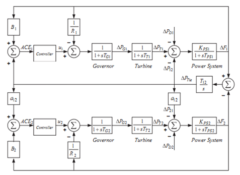
The dynamic model of AGC for an interconnected two-area system [5, 7, 9] is shown in Figure 1. Each area of the power system includes a speed governor, a turbine and a generator. Each area has three inputs and two outputs. Inputs are ΔPref control input (also showed by u), ΔPD is load perturbations, and ΔPTie crossing power error from tie line.
The outputs are the ΔF generator frequency and the area control error (ACE) presented in Eq. (16).
$\mathrm{B} \Delta \mathrm{F}+\Delta \mathrm{P}_{\mathrm{Tie}}=A C E$ (16)
where, B is the frequency displacement parameter. To simplify the frequency domain analysis, the conversion function is used to model each area element. The turbine conversion function is in accordance with (17).
Figure 1. Conversion function of double-district heating system
$G_{T}(S)=\frac{\Delta P_{T}(S)}{\Delta P_{V}(S)}=\frac{1}{1+S T_{T}}$ (17)
From Eq. (17), the governor conversion function will be as follows:
$G_{G}(S)=\frac{\Delta P_{V}(S)}{\Delta P_{G}(S)}=\frac{1}{1+S T_{G}}$ (18)
The speed governor system has two input ΔPref and ΔF and output ΔPG (s) as shown in Eq. (19).
$\Delta P_{G}(S)=\Delta P_{\text {ref }}(S)-\frac{1}{R} \Delta F(S)$ (19)
The generator and load are modeled with the conversion function shown in (20)
$G_{P}(S)=\frac{K_{P}}{1+S T_{P}}$ (20)
where, KP = 1/D and TP = 2H/fD.
The generator load system has two inputs ΔPT (S) and ΔPD (S) and one output ΔF (S) as shown in equating (21).
$\Delta F(S)=G_{P}(S)\left[\Delta P_{T}(S)-\Delta P_{D}(S)\right]$ (21)
The system under study as shown in Figure 1 is an interconnected two-area heating power system without reheating. This system has been extensively used in technical literature to design and analyze automatic load frequency control for interconnected districts. In Figure 1, B1 and B2 are frequency replacement parameters, ACE1 and ACE2 are errors of area control, u1 and u2 are control output from controller, R1 and R2 are parameters of setting speed governor in p.u. Hz, TG1 and TG2 governor time constants in seconds, ΔPV1 and ΔPV2 are changes in the Volvo governor position (p.u). TT1 and TT2 are the time constant of the turbines in seconds. ΔPT1 and ΔPT2 are the changes in the output power of the turbines. ΔPD1 and ΔPD2 are the demand variations of load; the ΔPTie is the development of the changes of crossing power from tie line (p.u). KPS1 and KPS2 are the power system gains, and TPS1 and TPS2 are the power system time constant per second, respectively. T12 is the coincidence factor, and ΔF1 and ΔF2 are the system frequency deviation in hertz. Nominal parameters of the investigated system are presented below [5, 7, 9].
$f=60 \mathrm{~Hz}, B_{1}=B_{2}=0.425 p \cdot u \cdot \frac{M W}{H z} ; R_{1}=R_{2}$
$=2.4 \frac{H z}{p \cdot u} ; T_{G 1}=T_{G 2}=0.08 s$
$T_{T 1}=T_{T 2}=0.3 s ; T_{P S 1}=T_{P S 2}=20 s ; T_{12}$$=0.545 P . u ; a_{12}=-1$
$K_{P S 1}=K_{P S 2}=\frac{120 H z}{p \cdot u}$
The degree of freedom of the control system is defined as the number of closed-loop conversion functions that can be independently set. Since various efficiency factors must be met in designing a control system and must be desirable in different ways, a two-degree of freedom control system has advantages over a single-degree of freedom control system [14]. The 2-DOF controller produces an output signal based on the difference between a reference signal and the measured output of the system. A weighted difference signal is calculated for each proportional multiplication, integral, and derivative operations according to predefined weight settings. The output of the controller is the sum of the output of the proportional multiplication, integral, and derivation operations on the related difference signals, where the reference signal of each operation is weighted according to the selected gain parameters [15].
The PI controller is often used in industry today. The non-derivative controller (D) is used when there is no need for rapid response, and they should be existed during the operation of noise processing and large perturbations and in the system with large transmission delays. The PID controller is used when stability and high response speed are required. Derivative mode improves system stability and enables us to increase proportional gain and reduce integral gain, which in turn increases the controller response speed.
According to the benefits stated, the use of PID controller [16, 19] and integral double-derivative controller (IDD) [6] for AGC has been reported in the technical literature. However, when the input signal has sharp edges, the derivative part generates unacceptable control signals as the plant unit input. Also, any noise in the input control signal leads to a large plant unit control input. These reasons cause to face with difficulty and complexity in practical applications. The practical solution to these problems is to put the filter-derivative in input and adjust its poles in way that no abnormality of response due to noise occurs due to its attenuating effect on high-frequency noise. To improve the efficiency when there is noise or random error in measuring process variables, a derivative filter is used. The derivative filter limits the large output shifts caused by the measured noise. The derivative filter can help to reduce the constant volatilities of the controller output, which can lead to the weariness of the control elements. Given the above, a derivative filter is used in this thesis.
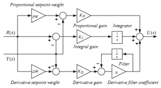
Figure 2. 2-DOF PID controller structure
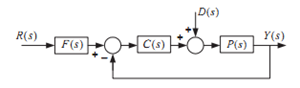
The structure of the parallel 2-DOF PID controller is shown in Figure 2 [15]. Where R (s) represents the reference signal, Y (s) represents the feedback from measured output of the system, and U (s) represents the output signal. KP, KI and KD are proportional, integral and derivative coefficients, respectively. PW and DW are the reference signal weights for the proportional and derivative controller and the N is derivative filter coefficient. A 2-DOF PID control system is shown in Figure 3. In this figure, C (s) is a controller with a degree of freedom, D (s) perturbations of laod, and F (s) act as a pre-filter on the reference signal.
Figure 3. 2-DOF PID controller
For a PID controller, two degrees of freedom C (s) and F (s) are given with the following equation:
$F(S)=\frac{\left(P W K_{P}+D W K_{D}\right) S^{2}+\left(P W K_{P} N+K_{1}\right) S+K_{1} N}{\left(K_{P}+K_{D} N\right) S^{2}+\left(K_{P} N+K_{1}\right) S+K_{1} N}$ (22)
$C(S)=\frac{\left(K_{P}+K_{D} N\right) S^{2}+\left(K_{P} N+K_{1}\right) S+K_{1} N}{S(S+N)}$ (23)
To design a 2-DOF PID controller based on a modern innovative optimization technique, the objective function is first defined according to the criteria and constraints. Selection of the objective function to optimize the controller is generally based on efficiency criteria that are dependent on the system response. In time domain systems, the desirable criteria are peak overshooting, rise time, setting time and steady state error. In the technical literature, the efficiency of different objective functions has been compared and reports indicate that ITAE is a better objective function in AGC studies [17, 18]. Therefore it is used as the objective function in this paper. Eq. (24) shows the expansion of the ITAE objective function.
$J=I T A E=\int_{0}^{t_{s i m}}\left(\left|\Delta F_{1}\right|+\left|\Delta F_{2}\right|+\left|\Delta P_{T i e}\right|\right)$ (24)
In Eq. (24), ΔF1 and ΔF2 are system frequency deviations; ΔPTie is the exponential changes of the power crossing tie lines, tsim is simulation time range. The constraints of problem are the boundaries of controller parameter. So the design problem can be formulated as the following optimization problem.
Minimize J
Subject to
$K_{P \min } \leq K_{P} \leq K_{P \max }, K_{I \min } \leq K_{I} \leq K_{I \max }$ and $K_{D \min } \leq K_{D} \leq K_{D \max }$
$P W_{\min } \leq P W \leq P W_{\max }, D W_{\min } \leq D W \leq D W_{\max }$ and $N_{\min } \leq N \leq N_{\max }$ (25)
where, J is the objective function and KP min, KP max, KI min, KI max, KD min and KD max are the minimum and maximum value of parameters, PWmin, PWmax, DWmin and DWmax are the minimum and maximum value of the reference signal weights of proportional and derivative controller. Nmin and Nmax are the minimum and maximum values of the derivative filter coefficient.
The PID controller parameters are selected in the range of -2.0 to 2.0. The time constant of the N-derived filter is generally greater than one. PW, DW and N should be in the range of 0 to 5 and 10 to 300.
The system model studied in Figure 1 has been stimulated in the MATLAB /SIMULINK software and the firefly algorithm is written as M.file. The model developed in a separate program has been simulated with an mfile by considering a 10% step change load in district 1. The objective function is computed in mfile and used in the optimization algorithm. For the efficiency of the firefly optimization algorithm, its parameters must be carefully selected. In this study, a population of NP= 100 with a maximum of 100 replicates has been considered. Simulation has been performed with a computer equipped with a Core i-5 CPU, with 2.5 GHz frequency and 4GB RAM in MATLAB (R2015a) software environment. The simulation has been performed 100 times and finally the best response between 100 times of the implementing program is selected as PI /PID / 2-DOF PID controller parameters. The best final responses from the 50 times of implementation are shown in Table 1.
Table 1. Optimized controller parameters with firefly algorithm
|
KP |
1.9 |
2.892 |
|
KI |
1.72 |
1.7476 |
|
KD |
0.2366 |
0.3236 |
|
N |
113.83 |
102.8251 |
|
PW |
0.4839 |
0.4859 |
|
DW |
1.1207 |
1.1334 |
Simulations are performed on a two-area system in three states.
• In the first state, no perturbation is applied to the system.
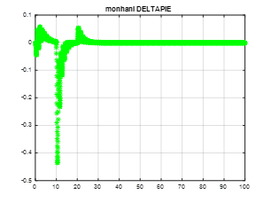
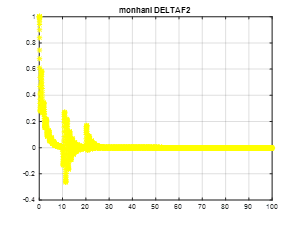
• In the second state, a perturbation of 1 perionite is applied to the first district in seconds 15.
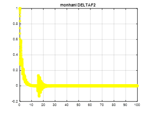
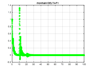
• In the third state, a perturbation of 2 perionites is applied to the first region in seconds 10 and 0.3 prionite in seconds 20 applied to the second state.
The results of the simulations in the three states mentioned above for tie power changes, frequency changes in the first area and frequency changes in the second area are presented in Figures 4 to 12.
In Table 2 in the first state of simulation, the results of the controller designed by Sahu et al. [14] are compared with the learning-based teaching algorithm with the firefly algorithm from the perturbation attenuation perspective. As we can see in the table, the settlement time of firefly algorithm is shorter, but settlement time of learning-based teaching algorithm is shorter.
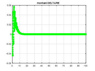
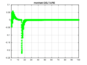
Figure 4. Tie crossing power changes in the first state
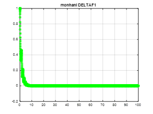
Figure 5. Frequency changes in the first area in the first state
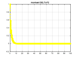
Figure 6. Frequency changes in the second area in the first state
Figure 7. Tie crossing power changes in the second state
Table 2. Comparison of results of Learning-Based Teaching Algorithm with Firefly Algorithm in first state
|
|
Firefly |
Learning-Based Teaching Algorithm |
|
Settlement time |
5.9407 |
5.3539 |
In Table 3 in the second state of simulation, the results of the controller designed in [14] are compared with the learning-based teaching algorithm with the firefly algorithm from the perturbation attenuation perspective. As we can see in the table, the settlement time of firefly algorithm is shorter.
Figure 8. Frequency changes in the first area in the second state
Figure 9. Frequency changes in the second area in the second state
Figure 10. Changes of tie crossing power in the third mode
Table 3. Comparison of results of Learning-Based Teaching Algorithm with Firefly Algorithm in second state
|
|
Firefly |
Learning-Based Teaching Algorithm |
|
Settlement time |
19.9508 |
22.5278 |
In Table 4, in the third state, the results of the controller designed by Sahu et al. [14] are compared with the learning-based teaching algorithm with the firefly algorithm from the perspective of perturbation attenuation. As we can see in the table, the settlement time of firefly algorithm is shorter.
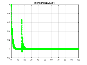
Figure 11. Frequency changes in the first area in the third state
Table 4. Comparison of results of Learning-Based Teaching Algorithm with Firefly Algorithm in Third State
|
|
Firefly |
Learning-Based Teaching Algorithm |
|
Settlement time |
22.0745 |
23.9354 |
Figure 12. Frequency changes in the second area in the third state
The relevant performance criterion, according to the ITAE value, has been considered for the frequency and standard deviation of the crossing power from tie line. It should be noted that the optimal values of the power system model controller parameters as shown above are obtained by optimization techniques and by minimizing the ITAE value that shown in Table 1. Sensitivity analysis was investigated to study the system's resistance to widespread changes in load changes conditions in the second and third states, the results are the appropriate response of the system behavior to this load perturbation.
It is evident that the eigenvalues for all states are on the left side of the pages. As it can be seen in this figure, changes in loading conditions under operation and system parameters have a negligible effect on the frequency deviation responses with the control parameters obtained from the nominal values. Therefore, it can be concluded that the proposed control strategy desirably shows a resistant control and optimal values that do not need to be reset by changing system loading or changing system parameters by using nominal loading values and nominal values of parameters.
In this paper, the firefly algorithm was used to solve the problem of automatic generation control. To solve this problem, the PID controller is generally considered as a degree of freedom that does not respond well to large load changes and perturbations. The use of a two-degree of freedom control structure to achieve the purpose of tracking and repelling the perturbation is helpful from the control perspective. Therefore, in this paper, the firefly optimization algorithm was used to find two-degrees of freedom controller parameters that have 6 parameters for each controller. It has been tried to use a 2-DOF PID controller as the AGC of an interconnected power system. The gains of the 2-DOF PID controller were set optimally using the ITAE objective function and the firefly optimization algorithm. First, a two-area heating power system was considered. Then, sensitivity analysis was performed to prove the resistance of the optimized control parameters to the wide changes of loading conditions. The results of this simulation show that the proposed method achieves better dynamic performance than the PID controller with a degree of freedom in this system. Finally, the dynamic response of power system under step load changes was investigated by the proposed method. It was found that the optimized 2-DOF PID controller with the proposed firefliy is very effective and it has a good dynamic performance.
[1] Saikia, L.C., Nanda, J., Mishra, S. (2011). Performance comparison of several classical controllers in AGC for multi-area interconnected thermal system. International Journal of Electrical Power & Energy Systems, 33(3): 394-401. https://doi.org/10.1016/j.ijepes.2010.08.036
[2] Rout, U.K., Sahu, R.K., Panda, S. (2013). Design and analysis of differential evolution algorithm based automatic generation control for interconnected power system. Ain Shams Engineering Journal, 4(3): 409-421. https://doi.org/10.1016/j.asej.2012.10.010
[3] Rakhshani, E. (2012). Intelligent linear-quadratic optimal output feedback regulator for a deregulated automatic generation control system. Electric Power Components and Systems, 40(5): 513-533. https://doi.org/10.1080/15325008.2011.647239
[4] Panda, S., Mohanty, B., Hota, P.K. (2013). Hybrid BFOA–PSO algorithm for automatic generation control of linear and nonlinear interconnected power systems. Applied Soft Computing, 13(12): 4718-4730. https://doi.org/10.1016/j.asoc.2013.07.021
[5] Ibraheem, Kumar, P., Hasan, N., Nizamuddin. (2012). Sub-optimal automatic generation control of interconnected power system using output vector feedback control strategy. Electric Power Components and Systems, 40(9): 977-994. https://doi.org/10.1080/15325008.2012.675802
[6] Pandey, S.K., Kishor, N., Mohanty, S.R. (2014). Frequency regulation in hybrid power system using iterative proportional-integral-derivative H∞ controller. Electric Power Components and Systems, 42(2): 132-148. https://doi.org/10.1080/15325008.2013.846438
[7] Parmar, K.S., Majhi, S., Kothari, D.P. (2012). Load frequency control of a realistic power system with multi-source power generation. International Journal of Electrical Power & Energy Systems, 42(1): 426-433. https://doi.org/10.1016/j.ijepes.2012.04.040
[8] Mohanty, B., Panda, S., Hota, P.K. (2014). Controller parameters tuning of differential evolution algorithm and its application to load frequency control of multi-source power system. International Journal of Electrical Power & Energy Systems, 54: 77-85. https://doi.org/10.1016/j.ijepes.2013.06.029
[9] Sánchez, J., Visioli, A., Dormido, S. (2011). A two-degree-of-freedom PI controller based on events. Journal of Process Control, 21(4): 639-651. https://doi.org/10.1016/j.jprocont.2010.12.001
[10] Sahu, R.K., Panda, S., Rout, U.K. (2013). DE optimized parallel 2-DOF PID controller for load frequency control of power system with governor dead-band nonlinearity. International Journal of Electrical Power & Energy Systems, 49: 19-33. https://doi.org/10.1016/j.ijepes.2012.12.009
[11] Sahu, R.K., Panda, S., Padhan, S. (2014). Optimal gravitational search algorithm for automatic generation control of interconnected power systems. Ain Shams Engineering Journal, 5(3): 721-733. https://doi.org/10.1016/j.asej.2014.02.004
[12] Shabani, H., Vahidi, B., Ebrahimpour, M. (2013). A robust PID controller based on imperialist competitive algorithm for load-frequency control of power systems. ISA Transactions, 52(1): 88-95. https://doi.org/10.1016/j.isatra.2012.09.008
[13] Tan, W. (2009). Unified tuning of PID load frequency controller for power systems via IMC. IEEE Transactions on Power Systems, 25(1): 341-350. https://doi.org/10.1109/TPWRS.2009.2036463
[14] Sahu, R.K., Panda, S., Rout, U.K., Sahoo, D.K. (2016). Teaching learning based optimization algorithm for automatic generation control of power system using 2-DOF PID controller. International Journal of Electrical Power & Energy Systems, 77: 287-301. https://doi.org/10.1016/j.ijepes.2015.11.082
[15] Kundur, P. (2008). Power System Stability and Control. 5th reprint. ed: New Delhi: Tata McGraw Hill.
[16] Bevrani, H. (2014). Robust power system frequency control. New York: Springer; https://doi.org/10.1007/978-3-319-07278-4
[17] Elgerd, O.I., Fosha, C.E. (1970). Optimum megawatt-frequency control of multiarea electric energy systems. IEEE Transactions on Power Apparatus and Systems, 89(4): 556-563. https://doi.org/10.1109/TPAS.1970.292602
[18] Ali, E.S., Abd-Elazim, S.M. (2011). Bacteria foraging optimization algorithm based load frequency controller for interconnected power system. International Journal of Electrical Power & Energy Systems, 33(3): 633-638. https://doi.org/10.1016/j.ijepes.2010.12.022
[19] Panda, S., Mohanty, B., Hota, P.K. (2013). Hybrid BFOA–PSO algorithm for automatic generation control of linear and nonlinear interconnected power systems. Applied Soft Computing, 13(12): 4718-4730. https://doi.org/10.1016/j.asoc.2013.07.021
[20] Zhao, Y.M., Xie, W.F., Tu, X.W. (2012). Performance-based parameter tuning method of model-driven PID control systems. ISA Transactions, 51(3): 393-399. https://doi.org/10.1016/j.isatra.2012.02.005
[21] Rao, R.V., Savsani, V.J., Vakharia, D.P. (2012). Teaching–learning-based optimization: An optimization method for continuous non-linear large scale problems. Information Sciences, 183(1): 1-15. https://doi.org/10.1016/j.ins.2011.08.006
[22] Debbarma, S., Saikia, L.C., Sinha, N. (2014). Automatic generation control using two degree of freedom fractional order PID controller. International Journal of Electrical Power & Energy Systems, 58: 120-129. https://doi.org/10.1016/j.ijepes.2014.01.011
[23] Pandey, S.K., Mohanty, S.R., Kishor, N. (2013). A literature survey on load–frequency control for conventional and distribution generation power systems. Renewable and Sustainable Energy Reviews, 25: 318-334. https://doi.org/10.1016/j.rser.2013.04.029
[24] Koisap, C., Kaitwanidvilai, S. (2009). A novel robust load frequency controller for a two area interconnected power system using LMI and compact genetic algorithms. In TENCON 2009-2009 IEEE Region 10 Conference, pp. 1-6. https://doi.org/10.1109/TENCON.2009.5395937
[25] Mishra, P., Mishra, S., Nanda, J., Sajith, K.V. (2011). Multilayer perceptron neural network (MLPNN) controller for automatic generation control of multiarea thermal system. In 2011 North American Power Symposium, pp. 1-7. https://doi.org/10.1109/NAPS.2011.6024887
[26] Anand, B., Jeyakumar, A.E. (2008). Load frequency control of hydro-thermal system with fuzzy logic controller considering boiler dynamics. In TENCON 2008-2008 IEEE Region 10 Conference, pp. 1-5. https://doi.org/10.1109/TENCON.2008.4766768
[27] El-Metwally, K.A. (2008). An adaptive fuzzy logic controller for a two area load frequency control problem. In 2008 12th International Middle-East Power System Conference, pp. 300-306. https://doi.org/10.1109/MEPCON.2008.4562327
[28] Shankar, R., Chatterjee, K., Chatterjee, T.K. (2012). Genetic algorithm based controller for load-frequency control of interconnected systems. In 2012 1st international conference on Recent Advances in Information Technology (RAIT), pp. 392-397. https://doi.org/10.1109/RAIT.2012.6194452
[29] Kumari, N., Jha, A.N. (2013). Particle Swarm optimization and gradient descent methods for optimization of PI controller for AGC of multi-area thermal-wind-hydro power plants. In 2013 UKSim 15th International Conference on Computer Modelling and Simulation, pp. 536-541. https://doi.org/10.1109/UKSim.2013.38
[30] Khodabakhshian, A., Hooshmand, R. (2010). A new PID controller design for automatic generation control of hydro power systems. International Journal of Electrical Power & Energy Systems, 32(5): 375-382. https://doi.org/10.1016/j.ijepes.2009.11.006