Investigations on Impact of Feature Normalization Techniques for Prediction of Hydro-Climatology Data Using Neural Network Backpropagation with Three Layer Hidden

Input data in the neural network back propagation (NNBP) architecture varies greatly and has different scales including static data patterns, decreased data patterns, increased data patterns, and even data patterns with extreme trends. The use of original data (raw data) to train neural networks can lead to convergence problems [1]. This will have implications for a high number of epochs and difficult networks to recognize data patterns. Therefore, the stage of normalization or standardization of data needs to be done before the data is trained in the NNBP architecture [2]. This normalization technique is included in the data preprocessing stage which will affect the accuracy of predictions significantly. The purpose of data normalization is to maintain all data value relationships appropriately in order to reduce the potential for bias in data [3]. It is in agreement with Nayak et al. [4] stating that data normalization aims (1) to minimize bias in neural networks from one feature to another, and (2) to accelerate training time by initiating the training process for each feature on the same scale.

Research on data normalization techniques as a stage of data preprocessing in NNBP has been widely carried out [4-12]. So, it can be known that normalization techniques include several data normalization techniques, namely, Z-score, min-max, mean-MAD, median-MAD, sigmoid, decimal scaling, tanh estimator, vector, and softmax. Panigrahi [11] has conducted experiments by training data on Wisconsin employment, monthly interest rates government bond yield 2-year securities, Reserve Bank of Australia, monthly milk production per cow in pounds, and temperature. He normalized the data with min-max, decimal scaling, median, vector, and Z-score techniques. The results showed that decimal scaling and vector techniques provide good accuracy results. This result is different from Tasdemir et al. [9] when calculated wind power performance and obtained that Z-score became the recommended normalization technique. 

Nayak et al. [4] when predicting stock markets, conducted data normalization experiments using min-max techniques, decimal scaling, Z-score, median, median-MAD, sigmoid, and tanh estimators. The results showed that the Z-score technique provided a good degree of accuracy and min-max could not be recommended. This result is also supported by Khond [6] when conducting data normalization experiments using min-max, softmax, decimal scaling, and Z-score techniques. He concluded that the Z-score normalization method is an effective and robust technique of data normalization when input data differ largely on the scale. In contrast, Nayak et al. [4] and Singh et al. [13] recommend the min-max technique to be used in the process of data normalization. Lastly, Eesa and Arabo [10] prefer the Mean-MAD and Median-MAD techniques in conducting normalization experiments of some unique client identifier (UCI) datasets.

The results of these studies provide different information related to recommendations for data normalization techniques that we should use when training-testing data. However, broadly speaking, more dominant normalization techniques are recommended, namely decimal scaling, Z-score, min-max, sigmoid, tanh estimators, median-MAD, and mean-MAD. Furthermore, when it is viewed from the writing of the formulas of these techniques, the researchers wrote with the same formula. However, for the min-max technique, each researcher gave a different formula. As example, Rohman et al. [14], Wang et al. [15], and Pradhan et al. [16] only use normalized data variables ($x_i^{\prime}$), data ($x_i$), maximum datum $\left(x_{i-\max }\right)$, and minimum datum $\left(x_{i-\min }\right)$ in data normalization with the formula:

$x_i^{\prime}=\frac{x_i-x_{i-\min }}{x_{i-\max } \quad-\quad x_{i-\min }}$    (1)

This formula is different from the formula used by Melesse [17] which multiplies $x_i^{\prime}$ by 0.99 plus 0.01. While, Singh et al. [13] multiply $x_i^{\prime}$ by 2 minus 1. Then, Lesnussa et al. [18] multiply $x_i^{\prime}$ by 0.8 plus 0.1. It is also different from Kumar et al. [19] that used the average variable ($\bar{x}_i$). Statistically, if we modify a variables and constants will certainly produce different calculation results. The min-max method is also used by Yang et al. [20] for stirling cryocooler predictions. Velasco et al. [21] utilized the method for the day-ahead base, intermediate, and peak load predictions. Elgin et al. [22] employed the method for bio-inspired classification. Lastly. Danpakdee and Songpan [23] used the method for skin image lesion classification.

Therefore, it is needed to be more in-depth experiments on the results of calculations for these data normalization techniques, especially the min-max technique compiled by researchers. Thus, it is clear that the min-max technique has a high degree of accuracy at intervals of 84.60%-96%. Hence, in this article, we apply statistical calculations to determine the mean square error (MSE) between actual data and normalization data. So that it can be seen simply which technique has the smallest MSE value. Then, we used all types of min-max techniques and other techniques including decimal scaling, Z-score, sigmoid, tanh estimators, median-MAD, and mean-MAD to data normalization. We also utilize two types of data with different patterns, namely rainfall data for seasonal data and air humidity data for stationary data. The results of this study are expected to provide new recommendations about the use of data normalization techniques to predict time series data using NNBP.

3.1 Selection of normalization techniques

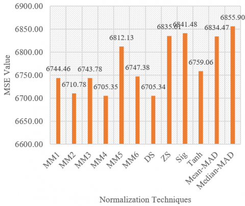
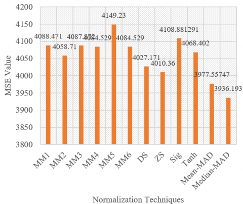
At this stage, we calculated descriptive statistical values of rainfall and air humidity data to determine the MSE value between actual data and data resulted from normalization, both rainfall data and air humidity data. The rainfall data obtained a minimum value of 0, a maximum of 401, a mean of 40.29, a median of 21, and a standard deviation of 49.93. Meanwhile, the air humidity data obtained a minimum value of 71, a maximum of 91, a mean of 82.64, a median of 83, and a standard deviation of 3.44. In the decimal scaling technique, researchers used a value of d of 2 for air humidity data and d of 3 for rainfall data. The results of the calculation of the MSE value between the actual data and the normalization data can be seen in Figure 1 and Figure 2.

Figure 1 provides information that five normalization techniques with small MSE values are MM1, MM2, MM3, MM4, and decimal scaling. Then, in Figure 2, we obtained a normalization technique with a small MSE value, namely MM2, decimal scaling, Z-score, Mean-MAD, and Median MAD. Thus, the five techniques were selected based on the case studies provided.

1.png

Figure 1. MSE value of air humidity (%)

2.png

Figure 2. MSE value of rainfall data (mm)

These five techniques were used in the data training process using a predetermined architecture. Because in computational algorithms the process of normalization is always followed by the process of de-normalization, the equation of each technique is obtained as follows.

- De-normalization for MM2

$x_i=2 \cdot\left(x^{\prime}-0.5\right) \cdot\left(x_{i-\max }-x_{i-\min }\right)+\bar{x}_i$       (2)

- De-normalization for Decimal scaling

$x_i=10^d \cdot x_i^{\prime}=10^2 \cdot x_i^{\prime}=100 \cdot x_i^{\prime}$      (3)

- De-normalization for Z-score

$x_i=x_i^{\prime} \cdot \sigma+\bar{x}_i$      (4)

- De-normalization for Mean-MAD

$x_i=x_i^{\prime} \cdot M A D\left(x_i\right)+\bar{x}_i$      (5)

- De-normalization for Median-MAD

$x_i=x_i^{\prime} \cdot MAD\left(x_i\right)+Median\left(x_i\right)$      (6)

Based on Table 1 and the de-normalization formula, computational scripts can be created using MATLAB as presented in Table 2.

3.2 Result of training data

Because there were two types of data, the data training process was carried out 10 times. Each training result was recorded and tabulated to see the number of epochs, MAE, and MSE. Graphs of actual data approaches and prediction data were also checked. The results of training data can be seen in Table 3.

Table 3 shows that in the case of rainfall data, it can be known that Z-score normalization technique gives good results with epochs of 10, MAE of 0.051, and MSE of 0.004. The next normalization techniques were the median-MAD technique with MAE of 0.111 and MSE of 0.059, the mean-MAD technique with MAE of 0.264 and MSE of 0.107, the min-max technique (MM2) with MAE of 17,519 and MSE of 545.49, and finally decimal scaling technique with MAE of 22,163 and MSE of 977.9. Then, in the case of air humidity data, it can be known that Z-score technique gives good results with epochs of 7, MAE of 0.018, and MSE of 0.006. This result is almost the same as that of the mean-MAD technique with an epoch of 8 and MSE of 0.0004 which is smaller than the MSE value of the Z-score technique. The min-max technique in training rainfall data did not give good results. This was because rainfall data had different patterns in each period so the range and standard deviation values were very large, namely 401 and 49.93, respectively. However, when training air humidity data, MAE and MSE values already looked smaller compared to the normalization of rainfall data, because the range and standard deviation were 20 and 3.44, respectively. The actual data approach and prediction data on the normalization results of the Z-score technique can be seen in Figure 3 and Figure 4.

Table 2. Computational normalization techniques using MATLAB Scripts

Table 3. Result of data training based on normalization techniques

3.png

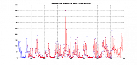
Figure 3. Actual data approach and prediction data of rainfall data (mm)

4.png

Figure 4. Actual data approach and prediction data of air humidity (%)

Figure 3 shows that the maximum rainfall in early November was 209.51 mm, and the minimum rainfall in mid-October was 5.01 mm. Generally, the forecast results show that in 2022 the intensity of rainfall in the Amperan area of Mataram city will be higher than the previous year. Furthermore, Figure 4 shows that the highest humidity occurs in October at 90%, while the lowest humidity occurs in September at 80%. Graphically, the distribution of the predicted data is already very close to the actual data. These results show that the Z-score technique gives good data normalization results before processing the data computationally, because of the Z-score is one of the data normalization techniques that determines how far a data is from its average value in its standard deviation units. It relates the whole to the average and its standard deviation this technique is able to make actual data errors and predictions become small. This is because the Z-score is able to reduce the epoch required by the architecture when the data training process takes place [8].