Hsiao-Hui Chen* | Udo Dietrich
© 2021 IIETA. This article is published by IIETA and is licensed under the CC BY 4.0 license (http://creativecommons.org/licenses/by/4.0/).
OPEN ACCESS
For the analysis of urban networks indicators, like average node degree, connectivity and betweenness centrality, are widely used. Their values are calculated for a catchment area of the network. This research investigates if and to what extent the size of the catchment area influences the indicator’s values. A methodology for determining the size of catchment area is proposed and recommendations for its appropriate size for pedestrian network analysis are offered. For the mathematical deduction of the relationship between the size of the catchment area and the indicator values an idealized regular network is used as a reference model. We found that the size effect on indicator values is prominent. It decreases exponentially as the size of the catchment area increases. The size effect is notable until a side length of the catchment area that equals 50 times the average street length, while the variation is still acceptable if it is 30 to 40 times the average street length. The typical average street length in cities is about 100 meters, a catchment area larger than 4000 x 4000m2 is not necessary. This reference model can also be used to evaluate real networks and to compare them with an idealized case.
average street length, catchment area, edge effect, network analysis, node degree, size effect
1.1 The challenge
When evaluating the real-world spatial networks, the central point and the catchment area around it need to be defined before carrying out network analysis, so that the indicators of different networks can be compared with each other. However, the real-world spatial networks are not strictly discreet systems and the boundaries of their catchment areas are often arbitrarily defined. This arbitrarily defined size of the catchment area often exerts significant distortion on the values of network indicators [1-6] for the following reasons.
If the size of the catchment area is too large, it is more likely that it contains multiple sub-networks or sub-structures with different characteristics. In other words, the mixed characteristics of the entire network are often a combination of sub-structures, such as grids, trees, hubs and spokes, or lines structure. And each type of network structure may differ in complexity [7, 8]. Since the value of the indicator is the average value for the entire network, the complexities of the sub-structures within the network may affect the calculation of the indicator for the evaluation of the characteristics and attributes.
On the other hand, if the catchment area is too small, the network model excludes the characteristics beyond the arbitrarily defined boundary of the model. Since the analytic algorithms are relational, the world outside the catchment area of analysis still affects the world inside it and the movement patterns within [1].
Concerns over the size effect on the reliability or significance of the network analysis results have been expressed and shared by many researchers [1, 9-12]. They test the size effect on the performance of spatial network models by varying the threshold radius of the catchment area. For example, Yoshimura et al. [13] have investigated betweenness centrality with radius of the catchment area varying from 300 to 5000 meters with 100 meters step, and the results show that the indicator value is sensitive to the size of the catchment area. To be more specific, the indicator value of the same node or link in the network may change with the size of the catchment area. And this distortion is particularly pronounced for the nodes and links at the border of the catchment area [1, 14]. For example, Gil [1] has found that nodes or links near the center of the catchment area tend to have higher degree of betweenness centrality compared with those close to the border. Accordingly, this influence has been called the “edge effect” or “boundary effect” [1, 9, 10, 14].
In this research, we focus on the effect of size of the catchment area on the indicator value. This effect is hereafter referred to as the “size effect”.
1.2 Types of research where size effect should be considered
Consideration of the size effect may be particularly crucial in research projects associated with the following purposes.
1.2.1 Research aiming at comparing and classifying multiple networks distributed in different locations
For any comparative study, where more than one network is included, the size of the catchment area will either have to be identical or it must be examined as one of the factors that may explain the variation of the measurement values among the multiple networks.
1.2.2 Research requiring the distinction among different types of mobility networks based on the mode of transportation, such as the networks for pedestrian, cyclists or motorized vehicles
For example, “a small road segment in a residential area might be important for pedestrians, but it is almost negligible for motorized transportation. In this sense, the road segment should have at least two kinds of importance: one for pedestrians and the other for motorized transportation” [15]. In other words, the value of the indicator varies depending on whether the catchment area is at the human or vehicle scale. Without considering the size of the study area, the degree of betweenness centrality cannot represent multiple aspects of the city that is perceived by people in the real world [16]. To avoid these problems, Yoshimura et al. [13] propose that, in addition to the global betweenness centrality for the entire city, a set of local betweenness centrality values at a smaller neighborhood scale shall also be calculated.
1.2.3 Research where an area needs to be divided into sections of smaller size with regular shape
The city area is often divided into smaller units due to the structural complexity and size associated with the scale problem [17-19]. For example, the analysis of connectivity of the road and street network structure is often conducted with the application of topological measures and typically requires that a large geographical space be divided into smaller parts with regular shape [8]. In a recent study, in order to determine the size of the catchment area on the value of the selected measures, Soczówka et al. [8] have carried out a comparative analysis by dividing the analyzed area into different sizes with regular shape and comparing the values of connectivity measurements of the road and street network structure. In such a case, the size of a single basic catchment area is very important because it can significantly affect the computational results of these measures.
1.2.4 Research measuring the spatial accessibility
Arbitrary administrative boundaries (such as census tracts or block groups) are often used in the studies of spatial accessibility. The arbitrarily defined border may lead to a methodological limitation [20, 21] because, first of all, accessibility involves movement and a given boundary does not actually prevent people or vehicles traveling across the border from reaching the facilities, services, amenities or any points of interest [22]. Secondly, a given boundary may exclude behavior outside the catchment area [12, 20-22, 23-31]. Thirdly, the resource or services beyond a defined arbitrary boundary may influence the behavior within the catchment area [27]. Many research projects studying the spatial accessibility have pointed out the risk that the accessibility of facilities may be biased [22, 25, 27, 32] or under-reported [12, 23, 28, 29, 33] because “areas close to the boundary may be classified as having poor geographic access even though they may in fact be proximate to resources across the boundary” [34].
1.3 Proposed solutions for mitigating the distortion
In an attempt to mitigate, contrast or diminish the distortions stemming from the size effect, the proposed features and principles underlying further classification can be broadly categorized into the following two approaches.
1.3.1 Adding a buffer zone with the assigned threshold radius
The first approach is to create buffer zones around the catchment area in order to compute the indicator value [1, 4, 35-37]. For example, the Python library OSMnx [38, 39] automatically creates a buffer of half a kilometer around the requested area so that each node has a correct street count. The buffer zones are then trimmed from the constructed network model. The indicator values of nodes and links within the buffer zone are excluded from the analysis because they are not reliable.
1.3.2 Using a homogeneous feature as the criterion for the division
Soczówka et al. [8] propose to divide the city area into smaller catchment areas with homogeneous features before conducting the analysis. They suggest several possible criteria of the homogeneous features including, firstly, administrative criteria, such as administrative district boundaries; secondly, structural criteria, such as the spatial distribution of density of inhabitants in households; and, thirdly, technical and functional criteria, such as the public transport management system.
In short, any divisions and classifications of geographical space should define the boundary of the catchment area. In response to these considerations, the current research intends to contribute to this decision process and to quantify the effect on the value of the indicators by 1) investigating whether and to what extend indicators, such as the node degree, change with the size of the catchment area; 2) proposing a methodology to decide the size of the catchment area based on the average street length; and 3) offering the recommendation for the appropriate size of the catchment area for the investigation of pedestrian networks.
A theoretical model representing an idealized regular network (see Figure 1) has been created as a reference model for the clear mathematical deduction of the relationship between the size of the catchment area and the changes in the indicator values. This allows us to answer the following research questions in a more controlled environment, where the differences in the values of the indicator will only be caused by the size effect (This is not ignoring the fact that, in the case of real network, the size effect may still exist regardless of the size of the catchment area. Because a real network is not regular to eternity and, therefore, its characteristics change).
2.1 The investigated indicator
The indicator we have chosen to examine the size effect is the average node degree, k, which is expressed by
$k=2 \times \frac{M}{N}$ (1)
where, M refers to the total number of links and N refers to the total number of nodes. In addition, the average node degree provides the information of the network pattern and can also be used to evaluate the level of "gridness.". A network with a lot of nodes connecting to 4 links, i.e. k$\cong$4, means that the network is more likely to be grid-pattern. And "more-gridded cities have higher connectivity (i.e., higher node degrees, more four-way intersections, fewer dead-ends etc.) and less-winding street patterns"[39]. This means that, holding the number of nodes constant, if the average node degree of a real network is smaller than that of a grid-pattern network, the connectivity of the real network is worse than the connectivity of a grid-pattern network.
Before examining the size effect on the node degree, we need to provide some definitions concerning our theoretical model.
2.2 The theoretical mathematical model
For the investigation of the size effect, a real network might not be a good basis to be the reference for comparison. The main problem is that the size effect cannot be clearly separated from other effects. Therefore, a theoretical model for the prognosis of the size effect was created in order to provide the method of mathematical analysis of an idealized regular network. In this way, the differences in the values of the indicator will only be caused by the size effect. Our definition of an idealized network consists of the following components.
2.2.1 Definition of a single quadrat as the basic element
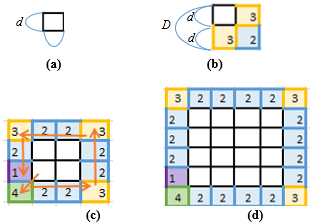
To illustrate the rules of how the network is created, we start with a network that is just a quadrat (square). As shown in (a) in Figure 2 and Table 1, a quadrat has four links as its boundary and it serve as the basic unit of the quadratic network with four nodes (N = 4) and four links (M = 4). We use d to refer to the length of a link in the network, which is also the side length of a quadrat.
2.2.2 Definition of a network
A quadrat is expanded and extended in the same quadratic pattern, as shown in (b), (c) and (d) in Figure 2 and Table 1. The size of the network is measured by the total number of nodes, N, and the total number of links, M. Element (b) in Figure 2 and Table 1 show that a network consisting of four quadrats has nine nodes (N = 9) and 12 links (M = 12).
2.2.3 Definition of a catchment area
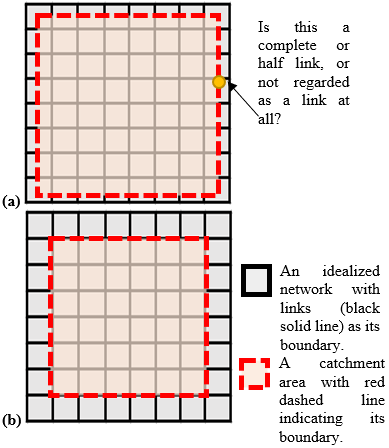
In the case of real networks, a network is different from a catchment area and the selected catchment area will be smaller than the entire network. As illustrated in Figure 1 (a) and (b), the black solid line indicates the links and also the boundary of a quadratic network and the red dashed line indicates the boundary of a catchment area. A catchment area is like the section that cuts off links connecting nodes from inside of the catchment area to nodes outside of the catchment area (In a real network, it is not necessarily the case that a catchment area cuts off links connecting nodes from inside of the catchment area to nodes outside of the catchment area. Sometimes, the boundary of the catchment area may coincidently lie exactly on a link as shown in Figure 1(b).). The link cut off by the catchment area could be counted as a complete or a half link. And the value of the indicator will be affected by how these links are counted. Alternatively, they might be excluded from the calculation altogether. For the purpose of this paper, we assume that these cut-off links are neglected and they are excluded from the calculation.
This means that the boundary of the catchment area consists of the links of the network as shown in Figure 1(b). Therefore, the side length of a catchment area, D, consists of one or multiple links of the network. And the size of the catchment area is D x D.
Figure 1. Abstracted expression of the boundaries of the idealized network and the catchment area
There can be two kinds of relationships between the network and the catchment area.
2.2.4 When the catchment area consists of one quadrat and D consists of single d (i.e. D = d)
In the case of the smallest catchment area (as shown in element (a) in Figure 2 and Table 1), there is only one quadrat and, therefore, the side length, D, of this catchment area equals to d. The size of the catchment area is D×D = d2. The network in this catchment area has 4 links (M = 4) and 4 nodes (N = 4). The node degree, k, is accordingly 2.
2.2.5 When the catchment area consists of multiple quadrats and D consists of multiple d
In element (b) in Figure 2 and Table 1, there are 4 quadrats and, therefore, the side length, D, of this catchment area equals to 2d. The size of the catchment area is D x D = 4d2. The network in this catchment area has 12 links. The total number of links, M, in this network is 12 and the total number of nodes, N, is 9. The node degree, k, is accordingly 2.67.
The relationship between the quadrat, the network and the catchment area of various sizes are summarized in Table 1 and it shows that, with the increasing side length, D, of the catchment area, the node degree, k, also increases. This means that there is a size effect on the indicator of node degree. This trend is noteworthy, so we break down the process into steps in order to investigate the details. The following discussion is divided into two parts: the additional links and the additional nodes.
Figure 2. Abstracted expression of the process of increasing the size of the catchment area
Table 1. Relationship between the quadrat, network and catchment area of various sizes
|
Elements in Figure 2 |
(a) |
(b) |
(c) |
(d) |
|
|
Number of quadrats |
1 |
4 |
16 |
36 |
|
|
Network |
Total number of links (M) |
4 |
12 |
40 |
84 |
|
Total number of nodes (N) |
4 |
9 |
25 |
49 |
|
|
Node degree (k) |
2 |
2.67 |
3.2 |
3.43 |
|
|
Catchment area |
Side length of catchment area (D) |
d |
2d |
4d |
6d |
|
Size of catchment area (D×D) |
d2 |
4d2 |
16d2 |
36d2 |
|
2.3 Process of increasing the size of the quadratic network
2.3.1 Increasing the number of links
Figure 2 presents the abstracted expression of the process of increasing the size of the catchment area. Figure 2 (a) shows one quadrat (square). The network with one quadrat is the smallest network.
Figure 2 (b) shows a network consists of 4 quadrats. To extend the network from (a) to (b) in Figure 2 and Table 1, three links are added to create the yellow quadrats. And then two more links are added to create the blue quadrat.
For the network in (c) in Figure 2 and Table 1, which is a network consists of 16 quadrats, we begin with a corner and, firstly, create the green quadrate with four links. Next, two more links are added to create another two blue quadrats. Thirdly, three links are added to create the yellow quadrat in the corner. Finally, these three steps are repeated until the final purple quadrate, which needs only one additional link to be created.
As the network becomes bigger and bigger, there are more and more blue quadrats, which are formed by two additional links, among the newly created quadrats. In other word, the number of blue quadrats increases much faster than other quadrats. Eventually this type of quadrat becomes more and more important and thus dominant the pattern of the increasing side length, D. Meanwhile, the yellow corner quadrat, which consists of 3 links, becomes less dominant.
2.3.2 Increasing the number of nodes
Since the blue quadrat is more dominant than the other types of quadrats on the increasing side length, D, the focus of the investigation is on this type of quadrats. For every blue quadrat, it takes two additional links to crease one additional node. Eventually the total number of nodes, N, will be half of the total number of links, M. Therefore,
$N=\frac{1}{2} M$ (2)
or, in other words,
$M=2 N$ (3)
This means that node degree, k, will eventually approach the final limit.
$k=2 \times \frac{M}{N}=2 \times \frac{2 N}{N}=4$ (4)
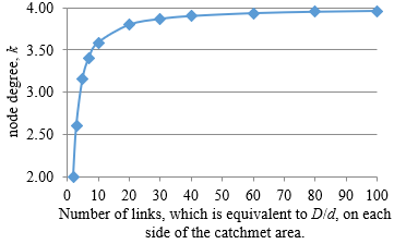
The results are shown in Figure 3 and Table 2.
Figure 3. Relationship between the value of the node degree, k, and the size of the catchment area, which is expressed by the number of links on each side of the catchment area
2.4 Appropriate size of the catchment area for pedestrians
For the investigations of pedestrian networks, it makes no sense to explore a large area. If we consider that the pedestrians’ maximum acceptable walking time is about 15 to 20 minutes, the size of the catchment area would be between 1500x1500m² to 2000x2000m². Also, following the findings regarding the size effect, the comparison between different “pedestrian” networks is only correct and thus possible if all catchment areas have the same size.
Table 2. Relationship between size of the catchment area and the values of indicators. The size of the catchment area is indicated by its side length, D, and D is indicated by the number of links, which is equivalent to D/d
|
Side length, D, of the catchment area |
Links in the network |
|||
|
Number of links on each side of the catchment area |
Total number of links, M |
Total additional links of base quadrat, indicated by the black links |
Total additional links required to create the new quadrat, indicated by colorful links |
|
|
1 |
4 |
4 |
4 |
|
|
2 |
12 |
4 |
8 |
|
|
4 |
40 |
12 |
28 |
|
|
6 |
84 |
40 |
44 |
|
|
8 |
144 |
84 |
60 |
|
|
10 |
220 |
144 |
76 |
|
|
12 |
312 |
220 |
92 |
|
|
14 |
420 |
312 |
108 |
|
|
16 |
544 |
420 |
124 |
|
|
18 |
684 |
544 |
140 |
|
|
20 |
840 |
684 |
156 |
|
|
40 |
3280 |
2964 |
316 |
|
|
50 |
5100 |
4704 |
396 |
|
|
100 |
20200 |
19404 |
796 |
|
|
Side length, D, of the catchment area |
New quadrat |
|||
|
Number of links on each side of the catchment area |
Number of new green quadrats formed by 4 additional links |
Number of new yellow quadrats formed by 3 additional links |
Number of new blue quadrats formed of 2 additional links |
Number of purple quadrats formed of 1 additional link |
|
1 |
1 |
0 |
0 |
0 |
|
2 |
0 |
2 |
1 |
0 |
|
4 |
1 |
3 |
7 |
1 |
|
6 |
1 |
3 |
15 |
1 |
|
8 |
1 |
3 |
23 |
1 |
|
10 |
1 |
3 |
31 |
1 |
|
12 |
1 |
3 |
39 |
1 |
|
14 |
1 |
3 |
47 |
1 |
|
16 |
1 |
3 |
55 |
1 |
|
18 |
1 |
3 |
63 |
1 |
|
20 |
1 |
3 |
71 |
1 |
|
40 |
1 |
3 |
151 |
1 |
|
50 |
1 |
3 |
191 |
1 |
|
100 |
1 |
3 |
391 |
1 |
|
Side length, D, of the catchment area |
Indicators |
|||
|
Number of links on each side of the catchment area |
Total number of nodes, N |
Node degree, k |
Nodes / area |
Area |
|
1 |
4 |
2.00 |
4.00 |
1 |
|
2 |
9 |
2.67 |
2.25 |
4 |
|
4 |
25 |
3.20 |
1.56 |
16 |
|
6 |
49 |
3.43 |
1.36 |
36 |
|
8 |
81 |
3.56 |
1.27 |
64 |
|
10 |
121 |
3.64 |
1.21 |
100 |
|
12 |
169 |
3.69 |
1.17 |
144 |
|
14 |
225 |
3.73 |
1.15 |
196 |
|
16 |
289 |
3.76 |
1.13 |
256 |
|
18 |
361 |
3.79 |
1.11 |
324 |
|
20 |
441 |
3.81 |
1.10 |
400 |
|
40 |
1681 |
3.90 |
1.05 |
1600 |
|
50 |
2601 |
3.92 |
1.04 |
2500 |
|
100 |
10201 |
3.96 |
1.02 |
10000 |
The benefit of investigating the size effect with a theoretical model is clear because, with the controlled condition, we can find out the scenario when the size effect is (nearly) saturated and deliver a correct prognosis about the total size of the network. Figure 3 shows the relationship between the value of the node degree, k, and the size of the catchment areas, which is expressed by the number of links on each side of the catchment area. It can be concluded that the size effect is very notable until the side length of the catchment area, D, equals 10 times of the length of the link, i.e. D = 10d. And it is still notable with a derivation of 3.8/4 = 5% when D = 20d. The derivation is reduced to 2.5% when D=40d, which can be regarded as a threshold and recommended as the size that is big enough to allow comparisons between different catchment areas and/or different networks. Eventually, it comes close to saturation where D = 50d. For values D >= 50d the node degree, k, reaches the ideal value of the extended network and the size does not play a role after that.
The principal implication of this theoretical model is twofold. First of all, the above investigation provides evidence to show that the size effect is remarkable and cannot be neglected until D = 40d.
Secondly, Table 3 shows the relationship between the average street length and the catchment area size range. The results offer a principle guideline for determining the size of the catchment area where the real network can be compared with the theoretical model. In the real street network, the average length of a street, which is the length of the link, d, in the theoretical model, is mostly between 50m and 100m. Assuming that d = 100m, the size of the selected catchment area has to be at least 20d x 20d = 2000x2000m2 in order to be able to compare it with the theoretical model. If the side length of the catchment area is 40d, i.e. 4000m, and the size of the catchment area is at least 4000x4000m2, the size effect will be even less significant in the theoretical model. Therefore, we provide the evidence to support that the lower and upper limits of the size of the catchment area should be 2000x2000m2 and 4000x4000m2.
Table 3. Recommendations for the lower and upper limits of the side length of the catchment area
|
Average street length, d |
50m |
100m |
|
Lower limit of the side length of the catchment area |
20d=1000m |
20d=2000m |
|
Upper limit of the side length of the catchment area |
40d=2000m |
40d=4000m |
|
Range of the sizes of catchment areas |
1000x1000m2 ~ 2000x2000m2 |
2000 x 2000m2 ~ 4000 x 4000m2 |
To sum up, the results in this research contribute to the argument that a catchment area with an area size that is too large would not be practical due to the following reasons.
First of all, the characteristics and patterns of the street networks in a real city may vary from quarter to quarter. For example, the characteristics of the network in the historical center would be different from its surrounding areas. Therefore, if the size of the catchment area is too big, the values of the indicators would reflect not the information about one type of network but rather about a sum of multiple types of networks in several neighboring and connected quarters. Such mixed information would be less valuable for investigating the relationship between the street network structure and the indicators or for classifying the street networks.
Secondly, the average street length can be one of the indicators for determining the size of the catchment area. According to our analysis, in the theoretical network, the size effect on the indicator is not very significant when the size of the catchment area is larger than 4000 x 4000m2. Therefore, any size larger than 4000 x 4000m2 would not be necessary.
Thirdly, the node degree of an idealized regular network changes with the size of the catchment area. But the variation becomes nearly neglectable when the size of the catchment area is larger than D = 40d and vanishes with D >= 50d. This means that, if the size of the catchment area of the real network is larger than D = 40d to 50d and the node degree is 4, the network pattern has a grid-like character. However, if the node degree of a real network is smaller than 4, its connectivity is worse than that of the theoretical grid-pattern network and vice versa.
Fourthly, we suggest that in all future investigations the size of the catchment area should be defined before carrying out further analysis.
Fifthly, when comparing the indicators of multiple catchment areas, all of the catchment areas should have the same size as long as D is less than 40d to 50d.
Finally, node degree has been chosen because its behavior can be calculated for the theoretical and idealized networks proposed in the current research in order to quantify and to demonstrate the size effect on the indicator values step by step. To what extent other indicators reach the saturation until the size effect vanishes should be part of further investigations. It would be interesting to test whether their threshold is also around D = 40 to 50 d. In future research, the analysis of the variability and the sensitivity of indicators shall facilitate decisions on which indicators should be used for a given size of the catchment area.
|
d |
length of a link in the network and also the side length of a quadrat, m |
|
D |
side length of a catchment area, m |
|
D×D |
size of catchment area |
|
k |
dimensionless average node degree |
|
M |
total number of links |
|
N |
total number of nodes |
[1] Greenberg, E., Natapov, A., Fisher-Gewirtzman, D. (2020). A physical effort-based model for pedestrian movement in topographic urban environments, Journal of Urban Design, 25(5): 1-22. https://doi.org/10.1080/13574809.2019.1632178
[2] Boeing, G. (2020). Planarity and street network representation in urban form analysis. Environment and Planning B: Urban Analytics and City Science, 47(5): 855-869. http://dx.doi.org/10.2139/ssrn.3191236
[3] Marshall, S., Gil, J., Kropf, K., Tomko, M., Figueiredo, L. (2018). Street network studies: from networks to models and their representations. Networks and Spatial Economics, 18: 735-749. https://doi.org/10.1007/s11067-018-9427-9
[4] Gil, J. (2017). Street network analysis “edge effects”: Examining the sensitivity of centrality measures to boundary conditions. Environment and Planning B Urban Analytics and City Science, 44(5): 819-836. https://doi.org/10.1177/0265813516650678
[5] Van Meter, E.M., Lawson, A.B., Colabianchi, N., Nichols, M., Hibbert, J., Porter, D.E., Liese, A.D. (2010). An evaluation of edge effects in nutritional accessibility and availability measures: A simulation study. International Journal of Health Geographics, 9(1): 40. https://doi.org/10.1186/1476-072X-9-40
[6] Pipley, B.D. (1981). Spatial Statistics. Wiley, New York.
[7] Żochowska, R., Soczówka, P. (2018). Analysis of selected structures of transportation network based on graph measures. Scientific Journal of Silesian University of Technology. Series Transport, 98: 223-233. https://doi.org/10.20858/sjsutst.2018.98.21
[8] Soczówka, P., Żochowska, R., Karoń, G. (2020). Method of the analysis of the connectivity of road. Computation, 8(2): 54. https://doi.org/10.3390/computation8020054
[9] Ratti, C. (2004). Space syntax: Some inconsistencies. Environment and Planning B: Planning and Design, 31(4): 487-499. https://doi.org/10.1068/b3019
[10] Park, H. (2009). Boundary effects on the intelligibility and predictability of spatial systems. Proceedings of the Seventh International Space Syntax Symposium, pp. 086: 1-086: 12. Royal Institute of Technology, Stockholm.
[11] Krafta, R. (1994). Modelling intraurban configurational development. Environment and Planning B: Planning and Design, 21(1): 67-82. https://doi.org/10.1068/b210067
[12] Sadler, R., Gilliland, J., Arku, G. (2011). An application of the edge effect in measuring accessibility to multiple food retailer types in Southwestern Ontario, Canada. International Journal of Health Geographics, 10(1): 34. https://doi.org/10.1186/1476-072X-10-34
[13] Yoshimura, Y., Santi, P., Arias, J.M., Zheng, S., Ratti, C. (2020). Spatial clustering: Influence of urban street networks on retail sales volumes. Environment and Planning B: Urban Analytics and City Science. https://doi.org/10.1177/2399808320954210
[14] Okabe, A., Sugihara, K. (2012). Spatial Analysis Along Networks: Statistical and Computational Methods. John Wiley & Sons.
[15] Yamaoka, K., Kumakoshi, Y., Yoshimura, Y. (2021). Local betweenness centrality analysis of 30 european cities. In: Geertman, S., Pettit, C., Goodspee, R., Staffans, A. (eds) Urban Informatics and Future Cities.
Springer International Publishing.
[16] Porta, S., Crucitti, P., Latora, V. (2006). The network analysis of urban streets: A primal approach. Environment and Planning B: Planning and Design, 33(5): 705-725. https://doi.org/10.1068/b32045
[17] Ahuja, N. (1983). On approaches to polygonal decomposition for hierarchical image representation. Computer Vision, Graphics and Image Processing, 24: 200-214. https://doi.org/10.1016/0734-189X(83)90043-9
[18] Bell, S., Diaz, B., Holroyd, F., Jackson, M. (1983). Spatially referenced methods of processing raster and vector data. Image and Vision Computing, 1: 211-220. https://doi.org/10.1016/0262-8856(83)90020-3
[19] Boots, B. (1980). Packing polygons: Some empirical evidence. Canadian Geographer, XXIV(24): 406-411. https://doi.org/10.1111/j.1541-0064.1980.tb00264.x
[20] Wan, N., Zhan, F.B., Zou, B., Chow, E. (2012). A relative spatial access assessment approach for analyzing potential spatial access to colorectal cancer services in Texas. Applied Geography, 32(2): 291-299. https://doi.org/10.1016/j.apgeog.2011.05.001
[21] Ngui, A.N., Apparicio, P. (2011). Optimizing the two-step floating catchment area method for measuring spatial accessibility to medical clinics in Montreal. BMC Health Service Research, 11(166). https://doi.org/10.1186/1472-6963-11-166
[22] Fortney, P.D., Rost, J., Warren, J. (2000) Comparing alternative methods of measuring geographic access to health services. Health Services & Outcomes Research Methodology, 1: 173-184. https://doi.org/10.1023/A:1012545106828
[23] Salze, P., Banos, A., Oppert, J.M., Charreire, H., Casey, R., Simon, C., Chaix, B., Badariotti, D., Weber, C., (2011). Estimating spatial accessibility to facilities on the regional scale: An extended commuting-based interaction potential model. International Journal of Health Geographics, 10(2). https://doi.org/10.1186/1476-072X-10-2
[24] Luo, J., Tian, L.L., Luo, L., Yi, H., Wang, F.H. (2017) Two-step optimization for spatial accessibility improvement: A case study of health care planning in rural China. BioMed Research International: 1-12. https://doi.org/10.1155/2017/2094654
[25] Donohoe, J., Marshall, V., Tan, X., Camacho, F.T., Anderson, R., Balkrishnan, R. (2016). Evaluating and comparing methods for measuring spatial access to mammography centers in Appalachia. Health Services and Outcomes Research Methodology, 16(1): 22-40. https://doi.org/10.1007/s10742-016-0143-y
[26] Bissonnette, L., Wilson, K., Bell, S., Shah, T.I. (2012) Neighbourhoods and potential access to health care: The role of spatial and aspatial factors. Health Place, 18(4): 841-853. https://doi.org/10.1016/j.healthplace.2012.03.007
[27] Van Meter, E.M., Lawson, A.B., Colabianchi, N., Nichols, M., Hibbert, J., Porter, D.E., Liese, A.D. (2010) An evaluation of edge effects in nutritional accessibility and availability measures: A simulation study. International Journal of Health Geographics, 9(40). https://doi.org/10.1186/1476-072X-9-40
[28] Sharkey, J.R., Horel, S. (2008). Neighborhood socioeconomic deprivation and minority composition are associated with better potential spatial access to the ground-truthed food environment in a large rural area. Journal of Nutrition, 138(3): 620-627. https://doi.org/10.1093/jn/138.3.620
[29] Wang, F., Luo, W. (2005). Assessing spatial and nonspatial factors for healthcare access: towards an integrated approach to defining health professional shortage areas. Health Place, 11(2): 131-146. https://doi.org/10.1016/j.healthplace.2004.02.003
[30] Vidal Rodeiro, C.L., Lawson, A.B. (2005). An evaluation of the edge effects in disease map modelling. Computational Statistics & Data Analysis, 49(1): 45-62. https://doi.org/10.1016/j.csda.2004.05.012
[31] Jordan, H., Roderick, P., Martin, D., Barnett, S. (2004) Distance, rurality and the need for care: access to health services in South West England. International Journal of Health Geographics, 3(1): 21. https://doi.org/10.1186/1476-072X-3-21
[32] Iredale, R., Jones, L., Gray, J., Deaville, J. (2005). ‘The edge effect’: An exploratory study of some factors affecting referrals to cancer genetic services in rural Wales. Health Place, 11(3): 197-204. https://doi.org/10.1016/j.healthplace.2004.06.005
[33] Zhang, X.Y., Lu, H., Holt, J.B. (2011). Modeling spatial accessibility to parks: a national study. International Journal of Health Geographics, 10(31). https://doi.org/10.1186/1476-072X-10-31
[34] Gao, F., Kihal, W., Le Meur, N., Le Meur, N., Souris, M., Deguen, S. (2017). Does the edge effect impact on the measure of spatial accessibility to healthcare providers? International Journal of Health Geographics, 16(1): 46. https://doi.org/10.1186/s12942-017-0119-3
[35] Pezzica, C., Cutini, V., De Souza, C.B.D. (2019). Rapid configurational analysis using OSM data: towards the use of Space Syntax to orient post-disaster decision making. 12th International Space Syntax Symposium (12SSS), Beijing, China, pp. 147.1-147.18.
[36] Penn, A., Hillier, B., Banister, D., Xu, J. (1998). Configurational modelling of urban movement networks. Environment and Planning B: Planning and Design, 25: 59-84. https://doi.org/10.1068/b250059
[37] Hillier, B., Penn, A., Hanson, J., Grajewski, T., Xu, J. (1993). Natural movement: Or, configuration and attraction in urban pedestrian movement. Environment and Planning B: Planning and Design, 20: 29-66. https://doi.org/10.1068/b200029
[38] Boeing, G. (2017). OSMnx: New methods for acquiring, constructing, analyzing, and visualizing complex street networks. Computers, Environment and Urban Systems, 65: 126-139. https://doi.org/10.1016/j.compenvurbsys.2017.05.004
[39] Boeing, G. (2019). Urban spatial order: Street network orientation, configuration, and entropy. Applied Network Science, 4(67): 1-19. https://doi.org/10.1007/s41109-019-0189-1