Variation in Total Factor Productivity of Corn in 19 Main Producing Areas under the Constraint of Carbon Emissions

To cope with climate change and promote low-carbon sustainable agriculture, countries around the world are competing to improve the total factor productivity (TFP) of agriculture under the constraint of carbon emissions [1]. As the largest food crop in China, corn can be consumed as our daily food, animal feed, and raw materials of energy. It provides an important guarantee for the food security [2] and energy security of China. In 2015, the Chinese Ministry of Agriculture issued the Guiding Opinions on the Adjustment of Corn Structure in the Sickle Bend, highlighting the importance of increasing the TFP of corn to the sustainable development of the corn industry.

Yang and Lu [3] effectively measured and decomposed the TFP of corn by the traditional approach for TFP measurement. But, for the following reasons, some of their judgements and interpretations are incorrect: first, their research emphasizes the adaptation between inputs and outputs over the coordination among inputs, outputs, and environment; second, their research only considers desirable outputs like corn yield, failing to take account of undesirable outputs like carbon emissions [4].

The Malmquist-Luenberger (ML) index, which is based on the directional distance function (DDF), can measure the agricultural TFP under environmental constraints, and include both desirable and undesirable outputs into the analysis framework [5]. Some scholars [5, 6] have adopted the ML index to measure the TFP of China’s agriculture under the constraint of environmental protection, and examine the growth and changes of its components. However, the measured results varied with the measurement calibers and selected indices. Considering undesriable outputs, some scholars [7-11] also relied on the ML index to measure the TFPs in industry, macroeconomy, and public transport. Some other scholars [12-14] employed similar methods to measure the TFPs of logisitcs, ports and cattle farms in different regions with theconstraint of carbon emissions. In the context of sustainable development, Houshyar et al. [15] adopted data envolopment analysis (DEA) to measure the corn TFP in Iran, but did not discuss the corn TFP in China. Furthermore, a number of scholars held that the TFP under undesirable constraints can be improved by suitable policies, including  liberalization of argicultrual market [16], green building policy [17], and agricultural structure [18].

In this paper, a corn TFP measurement model is established and used to measure the TFP indices (2008-2018) of corn and its components in main corn producing areas of China. Then, the features and causes of the variation in corn TFP were analyzed through temporal comparison between the situations before and after 2015 and spatial comparison between the areas in and out of the Sickle Bend. On this basis, policy suggestions were provided to promote the low-carbon production and increase the TFP of corn and other crops.

3.1 Global analysis

Based on our corn TFP measurement model, the global corn TFPs of the 19 main producing areas in 2008-2018 were evaluated on MaxDEA. The evaluation was carried out with and without the constraint of carbon emissions. The global TFPs were further decomposed into the TECH and EFFCH. The evaluation results are listed in Table 2.

Without the constraint of carbon emissions, the corn TFP decreased by 2.85% annually, the TECH degraded by 3.99% annually, and EFFCH improved by 1.53% annually from 2008 to 2018. With constraint of carbon emissions, the corn TFP decreased by 3.02% annually, the TECH degraded by 4.80% annually, and EFFCH improved by 2.63% annually in the same period.

Taking 2015 as the dividing line, the corn TFP decreased first and then increased. The corn TFP declined from 2008 to 2015, as TECH regressed faster than the improvement of EFFCH; the corn TFP grew from 2015 to 2018, for the TECH progressed faster than the deterioration of EFFCH.

Table 2. Global corn TFPs and components in 2008-2018

Fare et al. [25] suggested that the carbon intensity of production can be determined by comparing the magnitude of the TFP with constraint of carbon emissions and that (TFP₁) without the constraint of carbon emissions. When all input factors are the same, TFP>TFP₁ means the desirable output grows faster than the undesirable output, indicating that the DMU realizes low-carbon production; otherwise, the DMU realizes high-carbon production. On this basis, it can be judged that China’s corn production was in high-carbon mode in 2008-2015, and low-carbon mode in 2015-2018.

3.2 Regional analysis

Similarly, the corn TFP of each of the 19 main producing areas was measured and decomposed. The measurement results are listed in Tables 3-5.

With constraint of carbon emissions, the mean TFPs in four regions, namely, Hebei, Inner Mongolia, Guangxi, and Shaanxi, were greater than 1, while those of the other 15 main producing areas were smaller than 1. The fastest growing TFP belongs to Hebei, whose mean TFP was 1.0160; the fastest declining TFP belongs to Hubei, whose mean TFP was 0.9120.

The corn TFPs in four regions (including Hebei) increased, as their EFFCHs improved faster than the regression of TECHs. By contrast, the corn TFPs in 15 regions decreased. Among them, the decrease in 4 regions, namely, Heilongjiang, Henan, Hubei, and Ningxia, results from the EFFCH deterioration and TECH regression; the decrease in the other 11 regions occurred as their EFFCHs improved slower than the regression of TECHs. Overall, under the constraint of carbon emissions, the growth of corn TFP in China is mainly dragged down by the slow TECH progress.

As shown in Tables 4 and 5, from 2008 to 2015, the corn production was in high-carbon mode in 13 main producing areas, and in low-carbon mode in 6 main producing areas; from 2015 to 2018, the corn production was in high-carbon mode in 8 main producing areas, and in low-carbon mode in 11 main producing areas. Therefore, the corn production in China is moving towards low-carbon mode.

Table 3. Regional corn TFPs and components in 2008-2018

Table 4. Production modes of main corn production areas in 2008-2015

Table 5. Production modes of main corn production areas in 2015-2018

The above analysis reveals the corn TFP in China, and the sptial and temporal features of its components. Referring the Fare et al.’s criteria, the low-carbon technology innovators (LCTIs) that dominate the efficient frontier of China’s annual corn production must satisfy:

$M L T E C H_{t}^{t+1}>1$       (2)

$\overrightarrow{D_{0}^{\mathrm{t}}}\left(\mathrm{x}^{t+1}, y^{t+1}, b^{t+1} ; y^{t+1},-b^{t+1}\right)<0$       (3)

$\overrightarrow{D_{0}^{t+1}}\left(x^{t+1}, y^{t+1}, b^{t+1} ; \quad y^{t+1},-b^{t+1}\right)=0$       (4)

Formula (2) indicates that the efficient frontier expands towards more good outputs and fewer bad outputs; formula (3) indicates that the technical structure of period t is not applicable to period t+1; formula (4) ensures that the LCTIs fall on the efficient frontier. The regions that satisfy all three conditions are the LCTIs that dominate corn production in China (Table 6).

According to the above meaurement, from 2008 to 2018, nine main corn producing areas were the LCTIs that domianting the efficient frontier of China’s corn production, including Hebei for 4 years, Heilongjiang for 4 years, Inner Mongolia for 3 years, and Sichuan for 3 years. This means these four regions have attached importance to environmental protection and the efficiency of resource utilization.

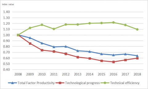
Figure 1 presents the variations in corn TFP, TECH, EFFCH with 2008 as the base year. It can be seen that, under the constraint of carbon emissions, China’s corn TFP exhibited a declining trend, except for the rises in 2012 and 2017, showing an annual decline of 6.39%. The TECH of China’s corn production regressed from 2008 to 2016 at an annual rate of 6.66%, and progressed 3.20% annually from 2016 to 2018. The EFFCH of China’s corn production increased with slight fluctuations; the annual increase was about 0.96%.

The above results indicate that, on average, the technical efficiency of China’s corn production has improved, and promoted the TFP of corn under the constraint of carbon emissions. However, the technical progress is slower than the regression of advanced technology, causing the corn TFP in China to decline with the constraint of carbon emissions.

Table 6. The LCTIs that dominate corn production in China (2008-2018)

1.png

Figure 1. Variations in corn TFP and its components under the constraint of carbon emissions

The following conclusions were drawn through measurement and analysis of the corn TFP in China:

(1) After 2015, the corn TFP in China was on the rise with constraint of carbon emissions, and the corn production was moving towards low-carbon mode, but exhibited huge regional difference.

(2) The policies on corn structure adjustment in the Sickle Band areas have effectively promoted the low-carbon production of corn in these areas, and improved the corn TFP.

(3) The growth of corn TFP in China is mainly bottlenecked by the slow technical progress.

Based on these findings, several suggestions were put forward:

(1) The policies on corn structure adjustment should be promoted to main corn producing areas outside the Sickle Band, as well as the main producing areas of other crops.

(2) The Chinese government should facilitate the exchange of low-carbon corn production experience, which could benefit the planting of other crops across the country.

(3) The Chinese government should also promote the technical progress on corn and other crops, which is the key to elevating crop TFPs.