Feng Xu![]() | Xinlin Li
| Xinlin Li![]() | Cuichan Wang
| Cuichan Wang![]() | Yansong Du
| Yansong Du![]() | Nana Hou
| Nana Hou![]() | Yichao Wang*
| Yichao Wang*![]()
© 2024 The authors. This article is published by IIETA and is licensed under the CC BY 4.0 license (http://creativecommons.org/licenses/by/4.0/).
OPEN ACCESS
The establishment of a high-fidelity simulation model for heating systems is crucial for practical guidance, as it serves predictive and evaluative purposes, offering accurate references for the operational management of actual engineering projects, thereby minimizing resource and cost wastage. This study, utilizing the Transient System Simulation Program (TRNSYS) software and focusing on an electric boiler water storage heating system in an elementary school, has developed a high-fidelity simulation model. Multiple TRNSYS (Types) modules were independently programmed, and the model's stability and precision were verified through error analysis. The model is capable of dynamically simulating the changes in supply and return water temperatures on both the storage and usage sides of the system under varying external environmental conditions and hydraulic states, achieving synchronous computation of the thermal and hydraulic characteristics of the heating system. The comparison and analysis of the temperature measurements at various system points against actual collected data revealed an average relative error of less than 5% across these measurements, indicating the simulation model's high accuracy and operational stability. It accurately and reliably reflects the thermal dynamics of the heating system, providing a reliable reference for practical application. This model is applicable for guiding the operational management of actual engineering projects and offers a scientific basis for subsequent system design and optimization.
electric boiler, Transient System Simulation Program dynamic simulation, error analysis, simulation accuracy
With the advancement of industrial levels and economic capabilities, the demands for regional heating have been continuously escalating [1]. In recent years, energy-saving and environmental protection policies such as coal-to-gas and coal-to-electricity conversions have been successively proposed, gradually increasing the attention to clean energy in regional heating schemes [2]. Electric boiler heating, due to its advantages of "no pollution, no emissions, and the full utilization of off-peak electricity [3]," has been widely applied in regional heating projects. Alongside the vigorous promotion of energy-saving and emission-reduction policies in China, the technical requirements for building heating to achieve higher efficiency and energy-saving targets have also heightened [4]. Under the premise of ensuring heating demand, enhancing the heating system's stability and reducing the operational energy consumption of heating have become particularly important.
During the heating engineering design phase, the selection of equipment usually relies on the maximum load that the equipment can withstand. However, in actual operation, equipment often operates under economic loads, frequently resulting in a mismatch between the actual operational load and the equipment's full-load operating characteristics, leading to the system operating in an inefficient state. This inefficiency can lead to poor heating and increased costs [5]. Therefore, there is a need for the establishment of a heating system simulation model that can reflect the system's thermal dynamic changes and provide a reliable basis for the actual operation of the heating system. Aunedi et al. [6] integrated models of different heat sources and thermal storage devices into energy system optimization models to assess their low-carbon heating potential under cost-effective conditions. Kilkis [7] established a low-temperature district heating system model with carbon reduction benefits to find the optimal capacity and temperature values for the equipment. Abugabbara et al. [8] proposed and designed a novel district heating simulation model, developed using the Modelica language, with simulation results indicating the model's applicability to the research and development of new heating systems. Zisopoulos et al. [9] utilized Aspen Plus Dynamics and Matlab/Simulink integration to simulate the energy storage part of integrated solar-driven thermal systems, demonstrating that the system can meet the energy needs of buildings. These researchers have constructed system simulation models using different software, employing simulation operation analysis to identify key factors affecting the system. Accurate simulation models can be used for designing new heating systems or optimizing existing ones. By modifying parameters and variables within the model, the performance and effects of different design schemes can be evaluated, allowing for the identification of the optimal system configuration and operational strategy before actual construction. For the simulation model of electric boiler water storage heating systems, software capable of simulating key parameter changes in the system, such as heat transfer, energy consumption, temperature variations, and accurately predicting and assessing the system's operational effectiveness is required.
The application of TRNSYS, renowned for its precise simulation, short cycle, and minimal output error, is extensively utilized in the optimization of Heating, Ventilation and Air Conditioning (HVAC) systems for energy saving and economic analysis [10]. TRNSYS is capable of segmenting the operation of system components into individual modules, has relatively open structure [11], and supports users to script module programs based on actual operational conditions for application within the software. Therefore, it is recognized as one of the most flexible building energy simulation software [12]. Rashad et al. [13] utilized TRNSYS for a comprehensive annual energy consumption analysis of a three-zone building, taking into account cooling and heating demands, thermal gains, and losses, resulting in the determination of the building's annual energy consumption. Chargui et al. [14] established a simulation model for a heat pump system using TRNSYS, conducting simulations to calculate the system's Coefficient of Performance (COP), energy consumption, and power supply. Dezhdar et al. [15] applied TRNSYS for transient optimization of a solar-wind multi-generation system, analyzing six determinants of system performance and subsequently employing the Response Surface Methodology to analyze simulation outcomes, thus identifying optimal system parameters.
Most researchers employing TRNSYS focus on areas such as building energy simulation [16], renewable energy system configuration [17], thermodynamic performance analysis [18], and optimization of control strategies [19]. The dynamic changes in hydraulic conditions present in actual systems are generally simplified or not considered in the software, due to the absence of corresponding computational modules in TRNSYS, leading to simulation results that may not fully represent actual operational outcomes. To establish a high-accuracy, high-stability simulation model for an electric boiler thermal storage heating system, this study, based on an electric boiler thermal storage system in a certain elementary school in Zhangjiakou, constructs a simulation model for its heating system using TRNSYS. Modules for pipe impedance and pump operating points, absent in TRNSYS, were independently developed and applied to ensure a closer alignment of simulation conditions with actual operational states. The accuracy of the model is gauged by comparing the simulated and actual measured temperatures at various system points, ensuring the model's applicability to real engineering projects and guiding actual operations.
The study is structured into three parts. The first part establishes a building energy consumption model, sequentially creating an accurate building energy model through steps such as constructing the building's geometric model, defining the parameters of building envelope materials, dividing thermal zones, and incorporating thermal gains. The second part involves constructing the simulation system, firstly by programming modules for pump operation points and pipe impedance, which are absent in TRNSYS. Based on this, a simulation system for the electric boiler thermal storage is constructed, reflecting actual system equipment parameters and operational strategies, allowing for concurrent hydraulic and thermal calculations to achieve simulation results that closely resemble actual conditions. The third part conducts an error analysis of the electric boiler thermal storage simulation system, comparing simulated data with actual measured data at various points to verify the model's accuracy and stability.
2.1 Overview of the building
In the context of a heating project for an elementary school in Zhangjiakou, a transition from coal to electric heating sources was undertaken. The heating structure, a four-story educational building, encompasses a total heating area of 3,064 m². The heating system integrates an electric boiler with a thermal storage tank, designed to store heat during off-peak electricity hours from 20:00 to 08:00, subsequently providing heating from 08:00 to 20:00. The indoor temperature is maintained at 10℃ during the night and 20℃ during the day, with radiators serving as the terminal heating devices.
2.2 Building thermal load model
The selection of the building for analysis involved gathering data on room areas, geometric information, and heated areas. A geometric physical model of the building was constructed using SketchUp software, allowing for the creation of separate thermal zones within the building's rooms. The physical model file was then exported and integrated into the TRNBuild module of TRNSYS. The thermal characteristics of the building were defined by setting parameters such as the type of building envelope, weather files for Zhangjiakou, and the orientation of the house, among other external influences. Internal gains, including heat emission from occupants and equipment, were input into the model based on room usage, ultimately facilitating the output of hourly energy consumption. The Zhangjiakou weather file was generated using Meteonorm8 software, providing a load file compatible with the TRNSYS-Type15 module. Internal load gains, driven primarily by lighting, personnel and equipment heat dissipation [20], were dynamically modelled with gain schedules due to their variability throughout the simulation.
Table 1. Parameters of building envelope structures
|
Envelope Structure |
Value (W/(m2·K)) |
|
Uexternal wall |
0.57 |
|
Uinternal wall |
0.68 |
|
Ufloor |
0.62 |
|
Uroof |
0.44 |
|
Uground floor |
0.44 |
|
Uwindow |
2.8 |
The application of TRNSYS software in computing building loads utilises a simplified building heat balance equation, encompassing thermal, moisture, and optical properties of the building. This considers various internal and external factors such as indoor-outdoor temperature differences, weather conditions, and solar radiation, enhancing the accuracy and reliability of building simulations. To expedite the computational process, certain simplifications were made, including the assumption of uniform temperature distribution within rooms and the neglect of local effects within the building.
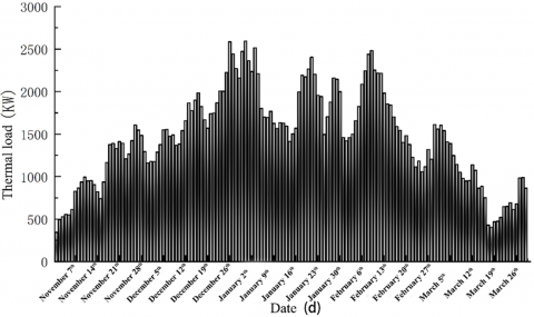
The computation of the model's energy consumption revealed the highest hourly energy consumption occurring at 01:00 on January 1st, amounting to 296.7 kW. Parameters for the building's envelope structures are detailed in Table 1, with a coupling diagram of the building energy model and influencing parameters illustrated in Figure 1. The required hourly thermal load of the building during the heating period is depicted in Figure 2 as well.
Initial indoor temperatures for rooms across all floors were set at 18℃, with a simulation time step of 1 hour during the thermal load output phase to facilitate the rapid generation of thermal load files.
Figure 1. Coupling diagram of the building model and influencing factors
Figure 2. Daily thermal load of the building during the heating season
3.1 Development of TRNSYS pipelines and water pump components
Within a heating system, heating equipment is connected to heat users through a heating network, which is responsible for transporting the thermal energy produced by the heat source to the heat users [21]. In practical engineering scenarios, adjustments in valve opening degrees by heat users within the system can lead to changes in the resistance coefficient of the heating network. Consequently, variations in the operating point of the water pump and the thermal medium flow rate of other heat users are observed [22]. Therefore, investigation into the dynamic characteristics of the heating system facilitates better prediction and control over the operational state of the system, ensuring maintenance of optimal hydraulic conditions. This reduces occurrences of hydraulic and thermal imbalances, minimizes unnecessary energy wastage, and thereby lowers operational energy consumption costs.
Owing to the absence of modules in TRNSYS software for dynamically changing pipe impedance and variable frequency water pumps, modules for valve opening degrees, pipe impedance, water pump conditions, and radiator types were developed using Visual C++6.0. These modules aim to enhance the model's accuracy by incorporating the impact of dynamic characteristics in the heating system.
a) Valve opening degree module
In the heating network, the degree of valve opening directly influences the network's impedance. By adjusting the valve opening degree appropriately, hydraulic balance in the heating system can be achieved, ensuring uniform distribution of hot water within the network and improving the efficiency and performance of the heating system. When partial adjustments to the heating network are required, changes in the valve opening degree at the user valve locations are typically made, altering the network's resistance characteristics. The calculation method for the pressure loss across a valve is as follows [23]:
$\Delta P_f=\frac{R^{2(1-X)}}{K_f^2} G_f^2$ (1)
where, $\Delta P_f$ represents the pressure loss across the valve in Pa; R is the adjustability ratio, the ratio of maximum flow to minimum regulation flow; $K_f$ denotes the relative opening of the regulating valve in percentage; $G_f$ is the valve's volumetric flow rate in m³/h; and X signifies the valve opening degree.
Given that valves act as accessories within the heating system's network, the impedance changes they induce are integrated into the overall resistance characteristics of the heating system's network.
b) Pipe impedance module
The inherent pipe module of TRNSYS, which encompasses parameters like the thermal loss coefficient, length, and inner diameter of pipes, does not account for the impedance characteristics of pipes. To bridge this gap, an output item detailing the pipe impedance characteristics was added. This modification facilitates the simulation of variable frequency pump operations under diverse conditions by providing essential input for determining the pump’s operating point. In outdoor heating networks, the flow of hot water within pipes predominantly resides in the square resistance zone [24], where the relationship between pressure drop ($\Delta P$) and flow rate (V) adheres to a quadratic law. The formula for calculating pipe pressure loss is as follows:
$\Delta P=S V^2$ (2)
$S=6.88 * 10^{-9} \frac{k^{0.25}}{d^{5.25}}\left(l+l_d\right) \rho$ (3)
$l_d=9.1 \frac{d^{1.25}}{k^{0.25}} \Sigma \xi$ (4)
where, S is the resistance number for the network calculation of pipe segments in Pa/(m³/h)²; k is the equivalent absolute roughness of the pipe's inner wall surface, with a general value of 0.5*10-3m for hot water networks; d is the internal diameter of the pipe in meters; l is the length of the pipe segment in meters; ld is the equivalent length of local resistance for the pipe segment; and ξ is the local resistance coefficient for the pipe segment.
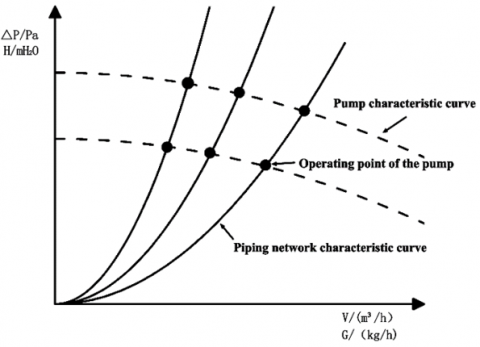
c) Pump operating condition point module
The operational condition point of a pump is determined by the combined characteristics of the piping and the pump itself, as illustrated in Figure 3. The two curves represent the characteristic curves of the piping network and the pump, with their intersection point defining the pump's operational condition. Should any one of these curves undergo a change, the operational condition of the pump will consequently alter. For instance, modifying the operating frequency of the pump or adjusting the opening degree of user valves will alter both the pump's characteristic curve and the piping characteristic curve. The new intersection of these two curves becomes the pump's revised operational condition, leading to changes in the hydraulic conditions of the piping network [25]. Not only will the total flow and pressure within the heating network vary, but changes in the impedance of specific pipe segments will also cause a redistribution of flow [8].
Figure 3. Characteristic curves of the pump and piping network
Given the limitations of the existing pump module in TRNSYS software, which fails to reflect the dynamic changes in the pump's operating point due to variations in pipeline impedance and pump frequency, the development of a new pump operating condition point module is necessitated. This module is designed to ascertain the operating condition points of variable frequency pumps under different scenarios.
The characteristic curve of the network can be derived from the previously developed pipeline impedance module. The pump characteristic curve equation can be sourced from the product manuals provided by pump manufacturers or deduced using the Lagrange quadratic interpolation formula based on actual operating data [26], represented in algebraic equation form as follows:
$H=a Q^2+b Q+c$ (5)
According to the law of similarity, changes in the rotational speed of variable frequency pumps result in alterations in pump head, described by the relationship [9]:
$\frac{H}{H_1}=\left(\frac{N}{N_1}\right)^2$ (6)
Moreover, the relationship between the rotational speed of variable frequency pumps and the frequency of the power supply is given by:
$N=60 \frac{f}{m}$ (7)
where, H denotes the pump head in meters; Q is the flow rate in m³/h; a, b, and c are coefficients derived from the pump characteristic curve equation; N and N1 represent the rated and actual rotational speeds of the pump in revolutions per minute, respectively; f stands for frequency in Hertz; and m is the number of magnetic pole pairs in the pump motor.
From the equations provided, the relationship between pump head and pump frequency can be discerned, allowing for the derivation of the characteristic curve equation for variable frequency pumps at different frequencies [26, 27]:
$H=\left(a Q^2+b Q+c\right) * i^2$ (8)
where, i represents the ratio of the pump's operating frequency to its rated frequency.
To ascertain the real-time energy consumption of variable frequency pumps at their operating points, a formula for calculating the pump shaft power was incorporated into the pump operating condition point module:
$P=\frac{\rho g Q H}{3600 \eta}$ (9)
where, P is the shaft power of the variable frequency pump in kW, $\rho$ is the density of the fluid in kg/m³, g is the acceleration due to gravity at 9.8 m/s², and $\eta$ is the total efficiency of the pump.
Consequently, the developed modules for valve opening degree, piping network impedance, and pump operating points have been designated as type334, type335, and type336, respectively. During usage, by inputting parameters such as segment length, inner diameter of the segment, and fitting coefficients of the pump characteristic curve, the operating condition values of the variable frequency pump, along with the shaft power at that operating point, can be directly outputted. This inclusion ensures that the impact of changes in hydraulic conditions on system operation is fully integrated into the simulation model, allowing for a closer alignment with actual operational conditions.
3.2 Simulation prototype
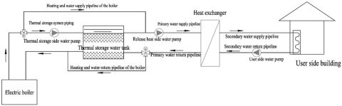
Figure 4 presents the process flow diagram of the electric boiler water thermal storage system for the elementary school, comprising an electric boiler thermal storage system, a primary water system, and a secondary water system. During the night-time thermal storage period, the electric boiler concurrently performs thermal storage and heating operations. During the day, when heat is released, the thermal storage water tank discharges heat to the user side. Heat is transferred from the primary water through a plate heat exchanger to the secondary water, and the temperature of the secondary water is adjusted by controlling the operation of the release heat pump and altering the frequency of the user side water pump when the secondary water temperature is excessively high. Throughout the heating season, based on the external temperatures during the early cold, severe cold, and late cold periods, the night-time electric boiler thermal storage temperatures are set at 56℃, 58℃, and 51℃, respectively. During the day, the remaining heat quantity in the thermal storage water tank is assessed by monitoring the return water temperature on the secondary side to determine if the residual heat is sufficient. If the residual heat is found to be insufficient, the electric boiler is activated between 12:00-13:00 to replenish heat to the thermal storage water tank.
Figure 4. Flow diagram of the water storage heating system of the electric boiler
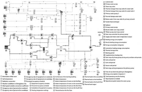
Figure 5. Simulation calculation model of the heating system
3.3 Construction of the system simulation model
Table 2. Inventory of equipment used in the system
|
No. |
Equipment Name |
Model |
Remarks |
|
1 |
Electric boiler |
350KW |
|
|
2 |
Thermal storage pump |
12.5m³/h-32m-2900r/min |
|
|
3 |
Tank discharge pump |
5m³/h-30m-2900r/min |
Efficiency: 69% |
|
4 |
Secondary side pump |
12.5m³/h-32m-2900r/min |
|
|
5 |
Plate heat exchanger |
PS102-10 |
|
|
6 |
Thermal storage tank |
64m³ |
|
Based on the operational strategy of the electric boiler water thermal storage system currently implemented at the school, the assembly of system equipment and controllers was conducted in TRNSYS-Studio. The construction process is detailed as follows: a) Importation of the required Type modules into the software interface, followed by sequential connection to construct the entire heating system model. b) The connection mode and parameters between modules were set to ensure that simulation runs could be conducted according to the actual process flow, with corresponding parameters inputted for each module, including properties, control strategies, and file sources. c) Importation and creation of connection components were performed, integrating the newly created hydraulic calculation module into the system, with sequential module connection and property input on the user side. d) During simulation runs, based on predefined control strategies, different modules within the software transmitted data through connected modules, conducting simulation calculations at set time steps. The simulation calculation model of the heating system is illustrated in Figure 5, with Table 2 and Table 3 respectively showing the actual equipment used in the system and the simulation equipment modules.
Table 3. Modules used in the simulation model
|
Module Name |
Module No. |
Module Name |
Module No. |
|
Electric boiler |
Type700 |
Radiator |
Type1214 |
|
Thermal storage pump |
Type110 |
Three-way diverting valve |
Type11f |
|
Tank discharge pump |
Type114 |
Temperature monitoring start-stop controller |
Type2b |
|
Secondary side pump |
Type114 |
Integrator |
Type24 |
|
Counterflow plate heat exchanger |
Type5b |
Valve opening degree module |
Type334 |
|
Thermal storage tank |
Type158 |
Piping impedance module |
Type335 |
|
Pump operating point module |
Type336 |
Output module |
Type65a |
|
Time control module |
Type14h |
|
|
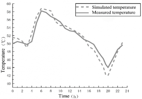
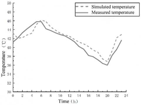
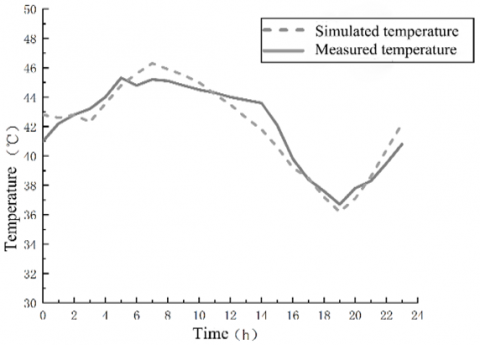
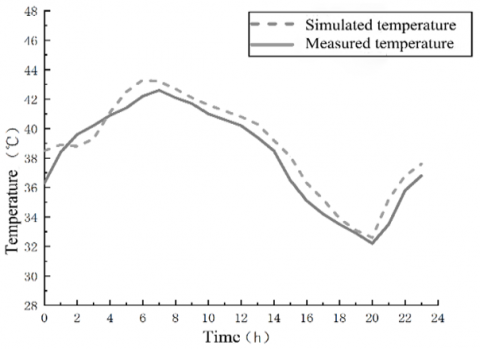
Upon the completion of the construction of the simulation model for the electric boiler thermal storage system, an output module was added to facilitate the comparison of the model's predictions with actual operational data. The output temperatures selected for this comparison were identified as the tank outlet temperature, tank return temperature, secondary side supply temperature, and secondary side return temperature on a typical day. The simulation step was set to 15 minutes, with output times designated at 24 hours and 168 hours, allowing for a more precise simulation of the variations in the tank outlet temperature.
Comparative analyses of the tank outlet temperature, tank return temperature, secondary side supply temperature, and secondary side return temperature on a typical day are presented in Figures 6, 7, 8, and 9, respectively.
Figure 6. Comparison of the tank outlet temperature simulation on a typical day
Figure 7. Comparison of the tank return temperature simulation on a typical day
Figure 8. Comparison of the secondary side supply temperature simulation on a typical day
From Figures 6, 7, 8, and 9, it is observed that the actual measured data largely align with the results simulated by the software, although certain discrepancies and fluctuations are noted, particularly in the graphs depicting the tank outlet temperature and the secondary side return temperature. Several factors are hypothesized to contribute to these observations: a) The thermal storage tank module in the software sets the heat loss rate as a constant value, whereas in actual conditions, the tank's heat loss rate varies with external temperature changes. b) The weather file used in the model differs from the conditions of the selected typical day, leading to temperature discrepancies during the heat discharge process of the tank. c) For simplification, the model does not account for heat losses in the heating pipes, which affects the secondary side return temperature in actual operation.
Figure 9. Comparison of the secondary side return temperature simulation on a typical day
Figure 10. Comparison of simulated versus actual tank outlet water temperatures over a typical week
The accuracy of the model is characterized by calculating the maximum error values and the average relative error values of the temperatures at various measurement points on a typical day. The calculation uses the actual measured temperatures and the simulated temperatures at each measurement point, hour by hour, to compute the relative error values; the largest difference in hourly temperature comparisons at each measurement point is taken as the maximum error value. The calculations reveal that the maximum error value for the tank outlet temperature on a typical day is 2.4℃, with an average relative error of 2.22%; for the tank return temperature, the maximum error value is 2.8℃, with an average relative error of 2.62%; for the secondary side supply temperature, the maximum error value is 1.9℃, with an average relative error of 1.77%; and for the secondary side return temperature, the maximum error value is 2.9℃, with an average relative error of 2.83%.
To comprehensively consider the effects of different weather conditions, load variations, and long-term operation of equipment on the simulation performance of the system, and to more accurately assess the simulation stability of the system, the tank outlet temperatures for the typical day and the actual measured temperatures for the week in which the typical day occurs are compared. Similarly, the maximum daily error values and average relative error values are calculated. The comparison of the simulated tank outlet temperatures for a typical week with actual measurements is shown in Figure 10, with the daily relative error values of the tank outlet temperature presented in Table 4.
Table 4. Daily relative error values between simulated and actual measured temperatures for a typical week
|
Simulated Tank Outlet Temperature |
Maximum Error Value |
Average Relative Error |
|
Day 1 |
2.4℃ |
2.22% |
|
Day 2 |
1.8℃ |
1.53% |
|
Day 3 |
2.8℃ |
2.33% |
|
Day 4 |
2.7℃ |
2.31% |
|
Day 5 |
1.6℃ |
1.44% |
|
Day 6 |
1.9℃ |
1.51% |
|
Day 7 |
2.2℃ |
1.82% |
From Figure 10, it is observed that as the daily minimum outdoor temperatures during the heating period progressively decrease, both the simulated and actual minimum outlet temperatures of the tank exhibit a downward trend. The daily maximum simulated outlet temperatures of the tank are consistently slightly higher than the actual measured temperatures. A slight deviation between the simulated and measured temperature curves of the tank's heat release process is noted, yet the overall trend remains fundamentally aligned. It is hypothesized that the source of error stems from the simplifications made by the TRNSYS software to ease model computations, typically assuming steady-state operation and neglecting transient effects during the start-up and shutdown phases of the electric boiler. These simplifications may lead to discrepancies between the simulated outcomes and actual conditions, hence temperature error points are predominantly concentrated around the periods of the electric boiler's start-up and shutdown. Table 4 indicates that the maximum error value in tank outlet temperatures within a week is 2.8℃, with the maximum average relative error being 2.33%.
Statistical analysis reveals that the average relative error values in the simulated temperatures of the aforementioned system do not exceed 5%, and the temperature differences remain within ±3℃. This indicates that the system simulation states established in the software closely match actual operational conditions, demonstrating high precision as well as long-term reliability and stability of the model. Therefore, it is concluded that the model possesses the requisite accuracy for dynamic temperature simulation in practical engineering applications.
In this study, a heating model of an electric boiler water storage heating system for a school was established based on the TRNSYS software. Several TRNSYS modules were independently developed to accommodate specific requirements, and a statistical analysis of the model's operational errors was conducted to verify its precision. The research yielded the following conclusions:
a) The TRNSYS (Types) modules, independently compiled using Visual C++6.0 software, were found to integrate effectively with the constructed heating system. This integration facilitated the acquisition of operating condition points for the system's water pumps, enabling simultaneous calculations of the thermal and hydraulic characteristics within the heating system. Such a methodology enhanced the accuracy of the simulation results.
b) Data derived from model simulations, when compared with actual measured data through error analysis, confirmed the accuracy and stability of the model. The established model is capable of simulating the operation of electric boiler thermal storage heating systems, offering guidance for real-world engineering operations. This provides a scientific basis for the design and optimization of systems in subsequent studies.
c) Certain assumptions made during the simulation process introduced limitations to the simulation results. For instance, the accuracy of weather data could cause fluctuations in the outcomes of the simulated system; assumptions regarding building usage patterns and human behavior as internal gains could limit the universality of the model's results under certain conditions. To further enhance the model's accuracy, the reliability of input data within the model needs to be ensured.
This work is supported by the Central Guidance of Local Science and Technology Development Funds Project—Research and Demonstration of Intelligent Control of Thermal Storage Heating System Based on Decoupling of Storage and Supply (Grant No.: 216Z6201G) and the Open Topics of Hebei Province Data Center Phase Change Thermal Management Technology Innovation Center (Grant No.: SKF-2022-02).
[1] Colmenar-Santos, A., Rosales-Asensio, E., Borge-Diez, D., Blanes-Peiró, J.J. (2016). District heating and cogeneration in the EU-28: Current situation, potential and proposed energy strategy for its generalisation. Renewable and Sustainable Energy Reviews, 62: 621-639. https://doi.org/10.1016/j.rser.2016.05.004
[2] Brinkley, C. (2018). The conundrum of combustible clean energy: Sweden's history of siting district heating smokestacks in residential areas. Energy Policy, 120: 526-532. https://doi.org/10.1016/j.enpol.2018.05.059
[3] Akhtari, M.R., Shayegh, I., Karimi, N. (2020). Techno-economic assessment and optimization of a hybrid renewable earth-air heat exchanger coupled with electric boiler, hydrogen, wind and PV configurations. Renewable Energy, 148: 839-851. https://doi.org/0.1016/j.renene.2012.10.169
[4] Wen, S., Liu, H. (2022). Research on energy conservation and carbon emission reduction effects and mechanism: Quasi-experimental evidence from China. Energy Policy, 169: 113180. https://doi.org/10.1016/j.enpol.2022.113180
[5] Zhang, C., Zai, X., Lu, M., Wang, R., Jing, Q., Zhan, C., Zhou, Z. (2021). Simulation and model validation of regional heating system based on TRNSYS. Building Science, 37(12):103-110. https://doi.org/10.13614/j.cnki.11-1962/tu.2021.12.15
[6] Aunedi, M., Olympios, A.V., Pantaleo, A.M., Markides, C.N., Strbac, G. (2023). System-driven design and integration of low-carbon domestic heating technologies. Renewable and Sustainable Energy Reviews, 187: 113695. https://doi.org/10.1016/j.rser.2023.113695
[7] Kilkis, B. (2021). An exergy-based minimum carbon footprint model for optimum equipment oversizing and temperature peaking in low-temperature district heating systems. Energy, 236: 121339. https://doi.org/10.1016/j.energy.2021.121339
[8] Abugabbara, M., Javed, S., Johansson, D. (2022). A simulation model for the design and analysis of district systems with simultaneous heating and cooling demands. Energy, 261: 125245. https://doi.org/10.1016/j.energy.2022.125245
[9] Zisopoulos, G., Nesiadis, A., Atsonios, K., Nikolopoulos, N., Stitou, D., Coca-Ortegón, A. (2021). Conceptual design and dynamic simulation of an integrated solar driven thermal system with thermochemical energy storage for heating and cooling. Journal of Energy Storage, 41: 102870. https://doi.org/10.1016/j.est.2021.102870
[10] Tiwari, A.K., Gupta, S., Joshi, A.K., Raval, F., Sojitra, M. (2021). TRNSYS simulation of flat plate solar collector based water heating system in Indian climatic condition. Materials Today: Proceedings, 46(11): 5360-5365. https://doi.org/10.1016/j.matpr.2020.08.794
[11] Ahamed, M.S., Guo, H., Tanino, K. (2020). Modeling heating demands in a Chinese-style solar greenhouse using the transient building energy simulation model TRNSYS. Journal of Building Engineering, 29: 101114. https://doi.org/10.1016/j.jobe.2019.101114
[12] Wei, D., Zhang, L., Alotaibi, A.A., Fang, J., Alshahri, A.H., Almitani, K.H. (2022). Transient simulation and comparative assessment of a hydrogen production and storage system with solar and wind energy using TRNSYS. International Journal of Hydrogen Energy, 47(62): 26646-26653. https://doi.org/10.1016/j.ijhydene.2022.02.157
[13] Rashad, M., Żabnieńska-Góra, A., Norman, L., Jouhara, H. (2022). Analysis of energy demand in a residential building using TRNSYS. Energy, 254(B): 124357. https://doi.org/10.1016/j.energy.2022.124357
[14] Chargui, R., Sammouda, H., Farhat, A. (2012). Geothermal heat pump in heating mode: Modeling and simulation on TRNSYS. International Journal of Refrigeration, 35(7): 1824-1832. https://doi.org/10.1016/j.ijrefrig.2012.06.002
[15] Dezhdar, A., Assareh, E., Agarwal, N., Bedakhanian, A., Keykhah, S., Fard, G.Y., Zadsar, N., Lee, M. (2023). Transient optimization of a new solar-wind multi-generation system for hydrogen production, desalination, clean electricity, heating, cooling, and energy storage using TRNSYS. Renewable Energy, 208: 512-537. https://doi.org/10.1016/j.renene.2023.03.019
[16] Cao, J., Liu, J., Man, X. (2017). A united WRF/TRNSYS method for estimating the heating/cooling load for the thousand-meter scale megatall buildings. Applied Thermal Engineering, 114: 196-210. https://doi.org/10.1016/j.applthermaleng.2016.11.195
[17] Lebedeva, K., Migla, L., Odineca, T. (2023). Solar district heating system in Latvia: A case study. Journal of King Saud University-Science, 35(10): 102965. https://doi.org/10.1016/j.jksus.2023.102965
[18] Abbassi, Y., Baniasadi, E., Ahmadikia, H. (2022). Transient energy storage in phase change materials, development and simulation of a new TRNSYS component. Journal of Building Engineering, 50: 104188. https://doi.org/10.1016/j.jobe.2022.104188
[19] Lu, M., Zhang, C., Zhang, D., Wang, R., Zhou, Z., Zhan, C., Jing, Q. (2021). Operational optimization of district heating system based on an integrated model in TRNSYS. Energy and Buildings, 230: 110538. https://doi.org/10.1016/j.enbuild.2020.110538
[20] El Bat, A.M.S., Romani, Z., Bozonnet, E., Draoui, A. (2021). Thermal impact of street canyon microclimate on building energy needs using TRNSYS: A case study of the city of Tangier in Morocco. Case Studies in Thermal Engineering, 24: 100834. https://doi.org/10.1016/j.csite.2020.100834
[21] Yokoyama, R., Kitano, H., Wakui, T. (2017). Optimal operation of heat supply systems with piping network. Energy, 137: 888-897. https://doi.org/10.1016/j.energy.2017.03.146
[22] Tian, X., Lin, X., Zhong, W., Zhou, Y. (2023). Sensitivity analysis and safety adjustment of the hydraulic condition in district heating networks. Energy and Buildings, 299: 113603. https://doi.org/10.1016/j.enbuild.2023.113603
[23] You, S., Mi, L., Wang, Y., Zhang, H., Zheng, X., Zheng, W. (2019). Unsteady hydraulic modeling and dynamic response analysis of a district heating network. Journal of Tianjin University: Science and Technology, 52(8): 849-856.
[24] Manservigi, L., Bahlawan, H., Losi, E., Morini, M., Spina, P.R., Venturini, M. (2022). A diagnostic approach for fault detection and identification in district heating networks. Energy, 251: 123988. https://doi.org/10.1016/j.energy.2022.123988
[25] Zhao, A., Dong, F., Xue, X., Xi, J.T., Wei, Y. (2023). Optimal control for hydraulic balance of secondary network in district heating system under distributed architecture. Energy and Buildings, 290: 113030. https://doi.org/10.1016/j.enbuild.2023.113030
[26] Thongkruer, P., Aree, P. (2023). Power-flow initialization of fixed-speed pump as turbines from their characteristic curves using unified Newton-Raphson approach. Electric Power Systems Research, 218: 109214. https://doi.org/10.1016/j.epsr.2023.109214
[27] Moreno, M.A., Planells, P., Córcoles, J.I., Tarjuelo, J.M., Carrión, P.A. (2009). Development of a new methodology to obtain the characteristic pump curves that minimize the total cost at pumping stations. Biosystems Engineering, 102(1): 95-105. https://doi.org/10.1016/j.biosystemseng.2008.09.024