Hussein M. Almyali*![]() | Zaid M.H. Al Dulaimi
| Zaid M.H. Al Dulaimi![]()
© 2023 IIETA. This article is published by IIETA and is licensed under the CC BY 4.0 license (http://creativecommons.org/licenses/by/4.0/).
OPEN ACCESS
The present study focuses on the examination of the combustion behavior of Iraqi LPG-air mixtures, flame propagation, and the tulip flame phenomenon in tubes. A new experimental facility was designed and constructed, featuring a complete setup comprising a combustion chamber unit, ignition unit, fuel injection and control unit, mixture preparation unit, and flame imaging unit. The combustion process was initiated through ignition by an electric spark, and both experimental measurements and numerical simulations were conducted using various turbulence models, including the realizable k-ε model, the k-ε model, and the Launder Sharma k-ε model. The study aimed to compare and validate the numerical results with empirical observations, specifically focusing on flame propagation velocity, peak pressures, and tulip flame formation. The investigation revealed that the k-ε model exhibited the closest agreement with experimental findings, accurately capturing flame propagation dynamics and tulip flame formation. However, discrepancies were noted in the numerical simulations, attributed to the absence of a wrinkling factor in the laminar combustion model, leading to smoother flame boundaries compared to experimental flames. The research highlighted the influence of turbulence on flame propagation beyond the tulip flame zone, necessitating further inquiries and model refinements to improve predictive capabilities. The findings affirm the appropriateness of the k-ε model in simulating the combustion process and provide valuable information for optimizing combustion efficiency and mitigating pollutant emissions. Future investigations will be essential to enhance turbulence models and advance the understanding of flame dynamics in confined environments. The comprehensive analysis of flame behavior presented in this study contributes to the advancement of combustion science and engineering, offering potential applications in various industrial and environmental settings.
combustion behavior, flame propagation, ILPG-air, tulip flame, turbulence models
Within the domain of combustion science, the investigation of premixed flame propagation in cylindrical conduits holds significant importance, owing to its far-reaching consequences for technological progress and industrial safety. The focal point of this investigation revolves around the captivating tulip flame phenomenon, an evident flame configuration observed within tubes possessing elevated aspect ratios and partial apertures. This phenomenon, which has undergone extensive research and has been documented in multiple studies [1-6], serves as a focal point for comprehending the intricate dynamics of flame behavior in confined spaces.
The exploration of the tulip flame phenomenon transcends a mere scholarly pursuit; it holds pragmatic implications across a diverse spectrum of applications, encompassing the optimization of combustion systems' efficacy and the assurance of industrial process safety. The phenomenon in controversy is a manifestation of intricate physical processes, wherein the interplay of velocities between unburnt and burnt gases engenders its distinct shape and behavior. The objective of this study is to thoroughly investigate the intricacies of these dynamics, utilizing the extensive collection of preexisting literature while generating novel perspectives and comprehensions. The behavior of the tulip flame within cylindrical conduits provides valuable insights into the overarching principles that govern flame propagation and stability. Through meticulous examination of this phenomenon [7].
Within the complex realm of analyzing flame propagation in cylindrical conduits, numerous critical variables and parameters arise as significant factors, as deduced from a comprehensive examination of existing literature. The conduit's aspect ratio, a geometric parameter, exerts a substantial influence on the occurrence of the tulip flame phenomenon, typically resulting in its formation [1-6]. The flame's shape and propagation speed are further influenced by the conduit's level of openness, wherein partial openness leads to alterations. The comprehension of flame behavior is contingent upon a thorough understanding of flow dynamics and fluid mechanics. The disparities in velocity between the unburnt and burnt gases play a crucial role in determining the shape of the tulip flame [4, 5]. The dynamics of vortices within the flame and the gases in its vicinity [6-11], in conjunction with hydrodynamic instabilities like Darrieus-Landau and Rayleigh-Taylor instabilities [8], have a significant influence on the deformation and stability of the flame [12-17].
The conduit experiences interactions with acoustic oscillations, which subsequently affect the flame's behavior in intricate manners [8, 9]. The morphology and propagation of the flame are influenced by various environmental and operational factors. These factors include the radius of the tube, the conditions of the tube walls (such as whether they exhibit free-slip or non-slip behavior and their temperature), and the characteristics of pressure waves. Previous studies [16, 17] have demonstrated the significant impact of these factors on the flame's behavior.
From a combustion and chemical perspective, the precise location of ignition within the conduit plays 1a crucial role in determining the behavior and spread of the flame [18, 19]. The equivalence ratio, which represents the ratio of fuel to oxidizer, plays a significant role in combustion dynamics and has a notable impact on flame speed and stability [18, 19]. Furthermore, the specific fuel type and its composition, including hydrogen-air blends or syngas combinations, play a crucial role in determining unique combustion characteristics [20].
The omprehensive analysis of literature indicates an intricate interplay of various factors that exert influence on the propagation of flames within cylindrical conduits. The dynamics encompass hydrodynamic, acoustic, and environmental factors, supported by theoretical and numerical models.
The thorough examination of flame behavior and its broader implications across scientific and industrial domains is of utmost importance. limited attention to experimental validation tests.
The investigation of flame propagation within cylindrical conduits has been a central area of focus in scientific research, particularly in the examination of the tulip flame phenomenon. The distinct flame morphology, primarily observed in tubes characterized by high aspect ratios and partial openness, has attracted significant interest in numerous investigations [1-5]. In accordance with recent research findings, it is postulated that the emergence of the tulip flame is not attributable to inherent instabilities within the flame front, but rather to a discrepancy in velocities between gases that have undergone combustion and those that have not [4, 5]. The aforementioned revelation, as proposed by Ponizy et al. [12], highlights the intricate nature of flame dynamics and its paramount importance in propelling industrial safety and technological advancement.
The hydrodynamic and acoustic influences are of paramount importance in this context. Prominent hydrodynamic phenomena, such as Darrieus-Landau instabilities [6, 7], acoustic oscillations [8, 9], vortex dynamics [10, 11], and the Rayleigh-Taylor instability, play a crucial role in influencing flame propagation. The comprehension and analysis of these elements are crucial in grasping the genesis and progression of the tulip flame, showcasing the intricate characteristics of flame dynamics within cylindrical conduits.
The phases of flame propagation encompass a series of distinct stages that occur during the combustion process. These stages can be classified as ignition, flame establishment, flame acceleration, and flame termination. Each phase plays a crucial role in the overall the advancement of flame propagation is characterized by discernible stages, as expounded upon by Clanet and Searby [14]. Commencing with a spheroidal combustion phenomenon, the flame undergoes a sequential progression into a 'finger flame' phase, experiences an increase in velocity, and ultimately assumes the form of a tulip as it decelerates. The phasic nature of flame behavior, as extensively examined by Xiao et al. [16, 17], elucidates the significant impact of pressure waves on the morphology of the tulip flame.
Environmental and operational factors are crucial considerations in the field of mechanical engineering. These factors encompass various elements that can significantly impact the design, performance, and longevity of mechanical systems and equipment. When designing mechanical systems, engineers must take into the flame dynamics are subject to substantial influence from various environmental and operational factors. The investigations conducted by Zheng et al. [18, 19] place significant emphasis on the influence of ignition position and equivalence ratio, specifically in hydrogen-air mixtures and syngas compositions, on the characteristics of combustion [20]. Furthermore, the impact of tube radius, wall conditions, and temperature on flame configuration has been a pivotal subject of investigation, as highlighted by Mohammadreza [21].
Theoretical models and numerical analysis are essential components of engineering practice. These methodologies allow engineers to analyze and predict the behavior of complex systems and structures. Theoretical models involve the development of mathematical equations and formulas that describe the physical phenomena and relationships within a system. These models Theoretical frameworks, as elucidated in previous studies [14, 22-32], establish a fundamental comprehension of flame dynamics, with a specific emphasis on the temporal variation of combustion gas volumes. In the current literature, there is a noticeable inclination towards numerical analysis, as observed in the publications of Al-Dulaimi [33] and Kumar [34]. However, it is important to acknowledge the continued necessity for experimental validation in order to supplement and corroborate these computational models. The progression of flame propagation investigation, commencing with Ellis [13] and furthered by Salamandra et al. [22], has played a pivotal role in molding our comprehension of flame morphology. The investigations explore the interplay between the flame front and the viscous flow, while also examining the impact of vortical fluid flow [24, 28-32]. These studies emphasize the importance of flame morphology in both physical and biological scenarios.
The present work aims to investigate the combustion characteristics of premixed fuel-air mixtures, specifically those involving LPG fuel. It seeks to fill the gap in comprehensive experimental measurements and numerical simulations to understand laminar flame speed and flame propagation behavior in these mixtures. The study's primary objectives are to experimentally measure the laminar flame speed of LPG and air mixtures, validate the results with numerical simulations, and visualize and analyze flame propagation behavior. The motivations behind this work stem from the practical importance of optimizing combustion processes involving LPG fuel, which is widely used in various applications. By gaining insights into combustion behavior and flame stability, the study can contribute to the design of efficient combustion systems and improve overall safety. Additionally, visualizing flame propagation will aid in understanding fundamental combustion processes. The findings from this study will advance combustion science and engineering and have practical implications for industries relying on LPG fuel.
The objective of this study is to accurately measure the flame speed and flame structure of partially premixed fuel-air mixtures, particularly involving LPG fuel, within the short measurement time available (a few milliseconds). To achieve this, a new experimental facility was designed and constructed at Al-Furat Al-Awsat Technical University, Technical Engineering College, Najaf, Mechanical Engineering department.
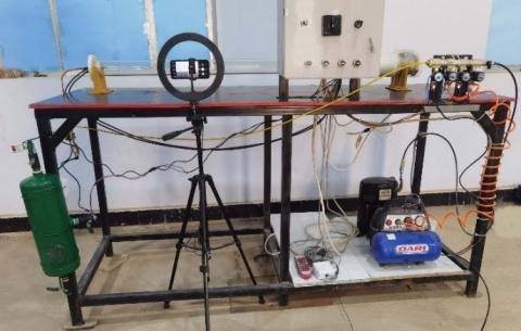
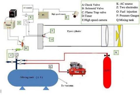
The experimental setup consists of the following units as seen in Figure 1.
Figure 1. Experimental rig
2.1 Mixture preparation processes
The mixture preparation processes include the following steps:
2.1.1 Flushing process of mixer
Air is admitted to the mixer for 3-5 minutes, repeated three times, to thoroughly flush any previous contents. The air admitting is performed at a moderate pressure to prevent unwanted temperature rise.
2.1.2 Vacuum process of mixer
All valves except the vacuum pump and vacuum gauge valve are closed. The vacuum pump evacuates the mixer until its pressure reaches approximately -0.92 bar.
2.1.3 Mixing process
The mixing process involves the following steps:
2.2 Combustion chamber preparation and combustion processes
One of the best methods used in combustion chamber preparation and combustion processes can be summarized as follows:
The experimental work outlined above aims to provide comprehensive measurements of the laminar flame speed and flame structure of partially premixed LPG and air mixtures. The data collected will be used to gain insights into the combustion behavior of these mixtures and to validate numerical simulations, ultimately contributing to advancements in combustion science and engineering, and practical implications for industries relying on LPG fuel.
2.3 Enhanced safety measures in LPG fuel experiments
In conducting experiments involving LPG fuel, a comprehensive safety protocol was paramount. Key measures included ensuring proper ventilation in the laboratory to prevent hazardous gas accumulation. Regular checks for leaks in the fuel supply system were conducted meticulously. Fire extinguishing equipment, including readily accessible fire extinguishers and emergency response protocols, were established. All personnel involved in the experiments underwent thorough safety training focused on handling LPG and emergency procedures. Additionally, the remote operation of experimental equipment was implemented where possible, to minimize direct human exposure to potential risks.
2.4 Data recording and measurement techniques
The experiments were designed to capture critical data for analyzing flame behavior. High-speed cameras paired with image analysis software were employed to measure flame speed accurately. The flame structure was visualized and analyzed using advanced flame imaging technology, enabling detailed observation of the flame front and its evolution. Pressure changes during the combustion process were monitored using sensitive pressure sensors installed within the combustion chamber. Temperature variations within the chamber were recorded using strategically placed thermocouples, ensuring comprehensive thermal profiling during each experiment.
2.5 Repetition for enhanced reliability
To ensure the reliability and accuracy of the experimental data, each setup underwent a minimum of five repeats for each reading. This repetition allowed for the verification of consistency across all experimental runs. Such rigorous testing protocols were crucial in establishing the reliability of the findings and ensuring that the results were representative and reproducible.
2.6 Observational overview of experimental results
The experiments yielded intriguing preliminary results. Distinct patterns in flame speed and structure were observed, which varied with changes in the equivalence ratio and pressure settings. These variations offered insights into the combustion efficiency of different fuel-air mixtures. Notably, under certain conditions, there was a transition observed from laminar to turbulent flame propagation. Additionally, significant pressure fluctuations were recorded within the combustion chamber, underscoring the dynamic nature of the combustion process. These observations are invaluable in enhancing the understanding of combustion behavior, particularly in the context of partially premixed LPG and air mixtures, and hold significant implications for optimizing combustion processes in industrial applications.
The utilization of computational fluid dynamics (CFD) methodologies has brought about a paradigm shift in the realm of scientific inquiry, bestowing upon its substantial merits in comparison to conventional laboratory experiments. The utilization of computational fluid dynamics (CFD) tools presents a cost-effective solution by obviating the necessity for costly physical testing apparatus and equipment. Furthermore, computational fluid dynamics (CFD) simulations afford researchers enhanced flexibility and command over experimental conditions, facilitating systematic and controlled investigations. Through the utilization of computational simulations on personal computing devices, scientists are able to computationally ascertain solutions to the fundamental equations governing a system and investigate an extensive array of hypothetical situations. The utilization of virtual experimentation greatly enhances the breadth and efficacy of scientific inquiry, enabling the exploration of various parameters and facilitating the juxtaposition of disparate scenarios. Nevertheless, it is imperative to duly recognize the intricacy inherent in computational fluid dynamics (CFD) methodologies, particularly in the context of simulating chemical reactions and turbulent flows. The computational demands of these simulations are significant, owing to the complexities inherent in the mathematical frameworks and the necessity for grids with high levels of resolution. Validating computational fluid dynamics (CFD) results against experimental data is of paramount importance in order to ascertain the veracity and precision of the obtained outcomes. Notwithstanding these considerations, computational fluid dynamics (CFD) tools afford researchers a potent and adaptable methodology to simulate and scrutinize the intricate dynamics of fluids, the transfer of thermal energy, and the intricate processes of combustion. This propels the advancement of scientific comprehension and engineering applications. In the current study, a computational fluid dynamics (CFD) model has been formulated and utilized to examine the dynamics and properties of flame propagation in diverse LPG/air mixtures under different blending circumstances. The utilization of chemical reactions and turbulent models would require a substantial allocation of computational resources. This chapter elucidates the computational aspects of the present study. The simulation of combustion processes involving mixtures has been accomplished through the utilization of Open FOAM code, which enables the resolution of intricate chemical reactions and turbulent models.
The present study has been implemented using the Xi Foam solver by considering the following assumptions for the current work:
The Xi Foam solver is used in the current simulation to solve the current combustion model. In this solver, the PDE is discretized using the finite volume method. The Xi Foam solver is an unsteady solver whose run duration and time step must be set so that Courant No. does not exceed the maximum value specified. A Courant number is a dimensionless value that represents the amount of time a particle spends in a single mesh cell. In this simulation, the maximal Courant number is set to 0.5, so:
Co.No $=\frac{u \Delta t}{\Delta x} \leq 0.5$. (1)
However, in the current configuration, an adjustable time step is enabled to prevent solution divergence during simulation. Combining the PISO (pressure-implicit split operator) and SIMPLE (semi-implicit method of the pressure-linked equation) algorithms, the PIMPLE algorithm is used to solve the pressure-velocity coupling. Second-order scheme discretization (LUST) is used to discretize the momentum equation, whereas Gauss limited linear is used to discretize the remaining equations: energy equation, turbulence model equation (the standard k-model is used in this work, as will be discussed in the following sections), and species conservation equations. The combustion model is enabled in the case file, and the reactions were properly set where there are different reactions based on the various cases investigated in this study, as demonstrated in the following section. The combustion within a chamber would be modeled using OpenFOAM code in the current numerical investigation. XiFoam solver will be used to solve the pertinent governing equations utilizing FVM (Finite Volume Method) with various discretization methods. Due to the inclusion of Multiphysics issues in the simulation modeling, the combustion numerical model is extremely complex. In addition, modeling reactions involving multiple species increases the number of relevant equations that must be solved. In addition, the turbulence model increases the complexity of the modeled problem. There are fundamental governing equations for fluid flow problems that must be implemented in the model first. To the main governing equations, such as the combustion and/or radiation sources, any additional model specifications can be added as a source or sink. Alternatively, scalar transport additives can be added as a distinct governing equation, such as the energy equation, multispecies equation, or turbulence model. All governing equations associated with numerical modeling are described in detail in the current section. The equation for mass conservation, also known as the continuity equation, the mass conservation equation is derived from the fundamental, well-known form of the continuity equation, which is written as:
$\frac{\partial \rho}{\partial t}+\frac{\partial\left(\rho u_j\right)}{\partial x_j}=0$ (2)
In the computational model, each equation is integral to understanding the fluid dynamics involved in flame propagation. It's crucial that all symbols used in these equations are clearly defined to ensure comprehensibility:
ρ: Density of the fluid (kg/m³)
t: Time (s)
uj: Velocity component in jth direction (m/s)
xj: Spatial coordinate in the jth direction (m)
The momentum equation, or what Navier-Stock named it, the definition of an equation is the equation that describes the flow characteristics (velocity and pressure) in all flow directions. Generally speaking, the final form of Navier-Stock's The x and y direction equation are:
$\begin{aligned} & \frac{\partial\left(\rho u_i\right)}{\partial t}+\frac{\partial\left(\rho u_i u_j\right)}{\partial x_j}=\frac{\partial P}{\partial x_i} +\frac{\partial}{\partial x_j}\left\{\mu\left(\frac{\partial u_i}{\partial x_j}+\frac{\partial u_j}{\partial x_i}-\left(\frac{2}{3} \delta_{i j} \frac{\partial u_k}{\partial x_k}\right)\right)\right\}\end{aligned}$ (3)
where, ui and δxi represent the velocity component and spatial distance in the flow direction, uj and δxj represent the velocity component and spatial distance in the other directions, P represents the pressure, and δij is the Kronecher Delta. is the mixture density that can be determined using the ideal gas law:
$\begin{gathered}P V=m R T \rightarrow \rho_{\text {mixture }}=\frac{P}{R T} \\ R=\frac{R_o}{M_{\text {ave }}} \\ M_{\text {ave }}=\frac{1}{\sum s \frac{Y_s}{M_s}}\end{gathered}$ (4)
where, Ro is the constant for all gases. Mave is the average molar mass of the mixture [35], where Ys and Ms are the mass fraction and molar mass for each chemical species, respectively, where the subscript s refers to the chemical species, and T is the temperature of the gas. Sutherland's law is used to calculate the gas dynamic viscosity as a function of temperature T in the present transport model:
$\mu=A_s \frac{\sqrt{T}}{T+T_s}$ (5)
where, As is the Sutherland coefficient and Ts is the Sutherland temperature; both are species constants.
The temperature is the most influential property in the combustion model's reactions. To calculate the temperature, the energy transport equation, also known as the energy conservation equation, must be implemented in the computational model. To include their effects in the final calculations, however, the combustion and radiation sources must be added to the energy transport equation. The energy conservation equation that includes the effects of combustion and radiation is as follows [35, 36]:
$\begin{aligned} \frac{\partial(\rho h)}{\partial t}+\frac{\partial\left(\rho h u_j\right)}{\partial x_j} & =\frac{\partial}{\partial x_j}\left\{\frac{\mu}{P r_h} \frac{\partial h}{\partial x_j}+\mu\left(\frac{1}{S c_s}-\frac{1}{P r_h}\right) \sum s h_s \frac{\partial Y_s}{\partial x_j}\right\} +\frac{\partial P}{\partial t}+S_{ {rad. }}+S_{ {comb. }}\end{aligned}$ (6)
Prh and Scs represent the mixture Prandtl Number and the species Schmidt Number, respectively, and Scomb. and Srad. are source variables added to the energy equation to account for combustion and radiation effects, where:
$P r_h=\frac{\mu c_p}{\lambda}$, while $S c_s=\frac{\mu}{\rho D_s}$
where, λ and Ds represent the thermal conductivity of the mélange and the diffusion coefficient of the species, respectively.
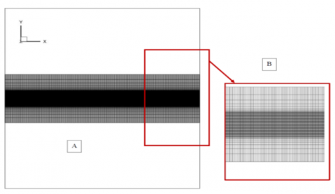
Open FOAM code has its own tool for mesh generation called “Block Mesh” where all the vertices that govern the domain are constructed to create the domain mesh blocks and boundaries. All these details are written as code in a journal file called “Block Mesh Dict”. However, in the current study, the whole geometrical domain of the studied control volume was constructed from structured mesh with hexa-blocks using the abovementioned tool. Thus, a uniform structured mesh was generated using different blocks as shown in Figure 2.
Figure 2. Computational domain and mesh details used in the current simulation: (a) the full domain, (b) zoomed view for a region of the domain
The computational domain has been generated such that the cells are larger on both sides while it becomes finer as it moves towards the center line to take the effects of flame into accounts, see Figure 3(b).
Five mesh sizes are set in the simulations to perform the mesh convergence study and approach the mesh independence, namely, 20000 cells (coarse mesh), 25000 cells (medium mesh), 30000 cells (fine mesh), 36000 cells (finer mesh size) and 64000 (more fine mesh size) are tested. Figure 3 demonstrates the temperature distribution along the center line above the flame tip position at the abovementioned five mesh sizes.
All are for the stoichiometric LPG/air mixture combination. It's worth mentioning that the difference in temperature values between the different mesh sizes appears in the figure to be greater than it is in reality since the figure is zoomed to be able to notice the difference, otherwise, the difference in the values is slight, especially between the fine & the very-fine mesh.
The figure also shows that the temperature distribution approaches its mesh independency at the very-fine mesh size where the curve in the very-fine mesh size matches the curve in the fine mesh size concluding that any further increase in the mesh would not affect the results significantly. Accordingly, the fine mesh size has been chosen for all the simulations of the present work.
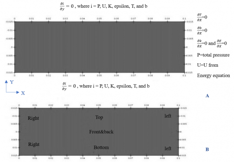
There are different types of boundary conditions used in the current computational model. Generally, the boundary conditions in the current numerical simulation are divided into four categories; boundary conditions involved in the turbulence model parameters, boundary conditions involved in the species of the chemical reaction, boundary conditions related to the energy transport parameters, and finally, the conditions involve the momentum equation parameters. Figure 3 shows the physical domain, whereas Figure 3(a) illustrates the domain pointer to it and the boundary conditions corresponding to each region. These boundary conditions were used for the solution of the problem through the discretization of the partial differential equations of the abovementioned model governing equations as shown in Table 1. Each condition was selected based on the following considerations:
Energy and Momentum Equations: Adjusted to reflect the thermal and fluid dynamic characteristics of the combustion process.
Validating the numerical model is essential to establish its reliability. This involves:
Such validation steps are crucial for confirming that the CFD model is a reliable tool for studying the dynamics of flame propagation in LPG/air mixtures.
Figure 3. The physical domain and its Boundary conditions: (a) types of Boundary conditions, (b) regions of the domain
Table 1. Boundary conditions specifications for main properties under each category of the governing equations
|
Turbulence Model Parameters |
|||||
|
|
Front and back |
Left |
Right |
Bottom |
Top |
|
∈ |
empty |
Symmetry Plane |
Symmetry Plane |
Symmetry Plane |
Symmetry Plane |
|
k |
empty |
Symmetry Plane |
Symmetry Plane |
Symmetry Plane |
Symmetry Plane |
|
nut |
empty |
Symmetry Plane |
Symmetry Plane |
Symmetry Plane |
Symmetry Plane |
|
∈ |
empty |
Symmetry Plane |
Symmetry Plane |
Symmetry Plane |
Symmetry Plane |
|
k |
empty |
Symmetry Plane |
Symmetry Plane |
Symmetry Plane |
Symmetry Plane |
|
Momentum and Continuity Parameters |
|||||
|
u |
empty |
Symmetry Plane |
Symmetry Plane |
Symmetry Plane |
Symmetry Plane |
|
p |
empty |
Symmetry Plane |
Symmetry Plane |
Symmetry Plane |
Symmetry Plane |
|
Energy Equation Parameters |
|||||
|
Alphat |
empty |
Symmetry Plane |
Symmetry Plane |
Symmetry Plane |
Symmetry Plane |
|
T |
empty |
Symmetry Plane |
Symmetry Plane |
Symmetry Plane |
Symmetry Plane |
|
Energy Equation Parameters |
|||||
|
b |
empty |
Symmetry Plane |
Symmetry Plane |
Symmetry Plane |
Symmetry Plane |
4.1 Validation
The process of ILPG-air explosion in a pipe was simulated utilizing several turbulence models, specifically the Realizable k-ε model, k-ε model, SST k-ω model, and Launder Sharma k-ε model. The study sought to establish a comparison between the simulation outcomes and empirical observations pertaining to the velocity at which a flame propagates, as depicted in Figure 4. Remarkably, the experimentally determined upper limit of flame propagation velocity was observed to be 14.4 meters per second. Among the various turbulence models employed, it was observed that the k-ε model exhibited the most favorable concurrence with the experimental findings. In the context of the numerical simulation, the combustion reaction transpired expeditiously following the ignition event, whereas the experimental arrangement encountered a temporal delay attributable to the initiation by means of an electric spark. Although the simulation exhibited accelerated flame propagation during the initial ignition phase, the velocity of the flame along the axis of the pipe remained consistent with the experimental observations. The simulation effectively utilized an adiabatic wall boundary condition, thereby conserving all thermal energy generated by the combustion process within the resulting products. In contrast, the experimental configuration involving a stainless-steel conduit encountered thermal dissipation, resulting in a depletion of energy. Notwithstanding this discrepancy, the flame propagation characteristics exhibited remarkable similarity in both instances. Despite the initial delay in the experimental flame acceleration and the gradual increase in flame speed, the maximum error in flame propagation speed was found to be less than 10%. Hence, it is inferred that the boundary condition exerted negligible influence on the overarching flame propagation pattern, and the k-ε model demonstrated its suitability in simulating the ILPG-air explosion phenomenon within the conduit. Figure 5 depicts the juxtaposition of experimental peak pressures and their corresponding calculated pressures at various measuring points along the pipe. Remarkably, the utmost pinnacle pressure was detected at the measurement location situated at the terminus of the conduit. The simulation employing the k-ε model yielded calculated pressures that exhibited a modest reduction in comparison to the experimental data, manifesting an average discrepancy of 11.9%. The observed discrepancy can be ascribed to the lack of energy dissipation within the simulated conduit. Nevertheless, it is worth noting that both the k-ε model and the Launder Sharma k-ε model exhibited a notable tendency to underestimate the maximum pressures. The average discrepancies between these models and the experimental findings were 16.75% and 24.12%, respectively. In light of these observations, the objective of this investigation is to ascertain the appropriateness and precision of the Realizable k-ε model in the context of simulating the propane-air explosion within the pipe. Additional inquiries are necessitated to comprehend and enhance the prognostic capacities of the turbulence models and their utilization in analogous circumstances.
Figure 4. Flame speed distribution along the pipe axis of various models and compared with experiential results
Figure 5. Flame pressure distribution along the pipe axis of various models and compared with experiential results
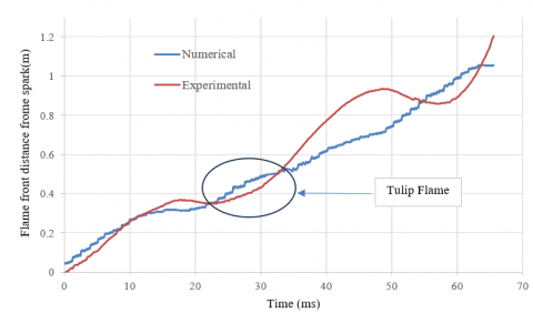
Figure 6. Flame front distance from spark of numerical and experimental work and compare with previous investigation
In Figure 6, a rigorous quantitative analysis is conducted to establish a correlation between the numerical outcomes and the empirical observations. The observed data demonstrates a congruence between the position and velocity of the flame within the first 32 milliseconds (prior to the formation of the tulip flame). This suggests that the model adequately represents the progression of the tulip flame. Nevertheless, subsequent to the occurrence of the tulip flame zone and until the temporal point t=54 ms, the numerical outcomes exhibit a significant underestimation in comparison to the empirical observations. The observed disparities between the numerical and experimental outcomes can be ascribed to the turbulence generated in the unburned mixture due to the expansion of the flame. The phenomenon of turbulence exerts a substantial influence on the dynamics of flame propagation, resulting in notable alterations in both the speed and behavior of the flame. In this scenario, it is plausible that the turbulent flow induced by the expansion of the flame could exert an impact on the propagation of the flame beyond the region characterized by the tulip flame. Consequently, this phenomenon could account for the disparities observed between the numerical forecasts and empirical observations. In order to enhance the precision of the numerical model and more effectively capture the dynamics of flame propagation, additional inquiries and refinements to the model are imperative. By incorporating a more comprehensive treatment of turbulence within the simulation, it is plausible to mitigate these discrepancies and augment the predictive prowess of the model pertaining to the entirety of flame propagation phenomenon. In the study conducted by Zakaria Movahedi [37], it was demonstrated that the spatial distribution and velocity of the flame within the first 30 milliseconds (prior to the formation of the tulip-shaped flame) exhibit a satisfactory level of concurrence. This suggests that the model employed in the investigation adequately represents the progression of the tulip flame. Nevertheless, subsequent to the occurrence of the tulip flame zone and extending until t=50 ms, a discernible incongruity in the temporal references pertaining to the noted disparities between the numerical and experimental outcomes becomes apparent. In my previous statement, I posited that the phenomenon of underestimation manifested itself within the temporal domain until t=50 ms. However, the supplementary data sourced from the scholarly work of Zakaria Movahedi elucidates that the aforementioned underestimation persisted until t=54 ms. Both sources exhibit concurrence in acknowledging the satisfactory correspondence between the numerical and experimental outcomes during the initial 30 milliseconds (prior to the formation of the tulip flame), thereby signifying a precise representation of the early progression of the flame. The phenomenon of the flame speed and location being underestimated subsequent to the tulip flame zone can be elucidated by considering the influence of turbulence within the unburned mixture induced by the expanding flame. The presence of turbulence can exert a substantial influence on the dynamics of flame propagation, resulting in notable modifications to the behavior and velocity of the flame. These alterations may serve as a plausible explanation for the disparities observed in the numerical forecasts extending beyond the tulip flame zone.
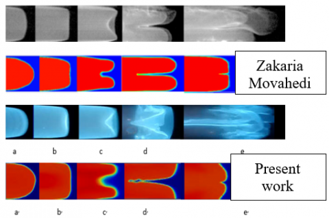
In Figure 7, a qualitative comparison is depicted, showcasing the tulip flame formation and the subsequent collapse of its lips. This comparison is made between the numerical approach utilizing a laminar flame model and the experimental methods employed. The experimental observations (frames a-e) portray the spatial location of the flame front as recorded by a high-speed camera in the course of experiments conducted on a homogeneous field of propane/air composition. On the contrary, the numerical outcomes (frames a´-e´) employ hues to depict the thermal gradient ranging from low-temperature gas (blue) to combusted substances (red) acquired through the simulation. In spite of certain disparities arising from the absence of a wrinkling component within the laminar combustion framework, the entirety of flame progression, encompassing the spherical morphology, subsequent flattening, formation of indentations, emergence of tulip-like structures, and eventual collapse of the flame lips, exhibits an exceedingly close resemblance between the experimental and numerical outcomes. The simulations successfully capture the fundamental qualitative aspects of the flame dynamics observed in the experiments. Nevertheless, it is pertinent to acknowledge that the numerical manifestation of the flame exhibits a greater degree of smoothness and reduced wrinkling in comparison to its experimental counterpart. The observed discrepancy can be attributed to the lack of the wrinkling factor in the laminar combustion model, which has a tendency to homogenize the flame boundaries and inhibit the emergence of intricate wrinkles observed in actual flames. Notwithstanding this constraint, the qualitative concurrence between the empirical and computational findings in apprehending the distinct phases of tulip flame genesis and lip collapse is noteworthy. The observed results affirm the general efficacy of the laminar flame model in accurately replicating fundamental characteristics of the tulip flame phenomenon, thereby offering significant understanding into the dynamics of the flame throughout these specific phases of combustion. The current study exhibits satisfactory concurrence with the observations made by Zakaria Movahedi in terms of both experimental and numerical outcomes. The juxtaposition of the two works elucidates congruent patterns and phenomena in diverse facets of the investigation, encompassing flame localization, velocity, and the dynamics of formation.
The experimental findings of this study exhibit similar patterns and properties as those observed by Zakaria Movahedi, thereby suggesting a high degree of consistency and reliability in the experimental configurations and data acquisition techniques employed. The congruence observed in the experimental results serves to bolster the level of certainty regarding the precision of the current study. Moreover, the quantitative outcomes obtained in the current investigation exhibit commendable concurrence with the numerical simulations conducted by Zakaria Movahedi. In spite of certain disparities arising from the lack of a wrinkle factor in the laminar combustion model, both investigations successfully capture fundamental qualitative aspects pertaining to the formation of the tulip flame and the subsequent collapse of its lips. The observed consistency in the results suggests that the numerical model employed in this study is well-suited for simulating and comprehending the flame's dynamics throughout these particular stages. The congruence between the empirical and computational outcomes of the current investigation and the study conducted by Zakaria Movahedi bolsters the veracity of the discoveries and fortifies the soundness of the utilized methodologies and frameworks. The observed consistency in the obtained data from both studies serves as a significant validation, affirming the accuracy and reliability of the collected information. This validation, in turn, contributes to the broader comprehension of the propane-air explosion process and the tulip flame phenomenon occurring within the pipe.
Figure 7. The validation between experimental work and numerical simulation of present and previous investigations
4.2 Flame propagation mechanism (Numerical investigation)
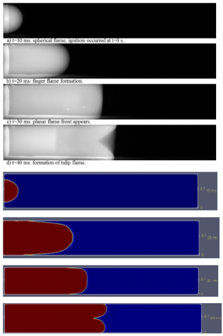
Flame propagation from time zero to the time of tulip generation involves the progression of the combustion front and the development of the flame structure over time. Initially, at time zero, the combustion process starts with the ignition of the fuel-air mixture. The flame front begins to propagate outward from the ignition source, driven by the heat released from the chemical reactions occurring within the mixture. As the flame front expands, it consumes the unburned fuel and air, creating a region of combustion. During this early stage of flame propagation, the flame front appears relatively smooth and compact, gradually advancing into the unburned mixture. As time progresses, the flame front encounters turbulence and flow disturbances within the combustible medium, leading to changes in its shape and structure. As the flame front approaches the time of tulip generation, typically at 0.04 seconds as mentioned, a distinctive phenomenon occurs. The flame front develops a tulip-like shape, characterized by a bulbous region at the flame tip. This tulip flame structure arises due to the interaction between the flame front and the surrounding turbulent flow. The turbulence induces local variations in fuel-air mixing and flame stabilization, leading to the formation of the tulip shape. The tulip flame structure is often associated with enhanced heat release and flame stability, which can have implications for combustion efficiency and pollutant emissions. Its presence indicates complex interactions between the flame front, turbulence, and fuel-air mixing processes [38].
Figure 8 serves as a visual representation that elucidates the intricate dynamics inherent in the combustion process, specifically pertaining to the mechanisms governing flame propagation. One remarkable phenomenon that has been observed in the depicted scenario is the emergence of a tulip-shaped flame precisely at the temporal mark of 0.04 seconds. The tulip flame exhibits a discernible morphology reminiscent of the floral structure of a tulip. The phenomenon arises when the combustion front undergoes propagation in a curvilinear fashion, thereby resulting in the emergence of a bulbous region at the apex of the flame. The distinctive flame structure observed is frequently linked to turbulent combustion scenarios, wherein the fluid dynamics exert a substantial influence on the configuration of the flame front. The phenomenon of the tulip flame holds significant intrigue owing to its profound influence on the optimization of combustion efficiency, mitigation of pollutant emissions, and preservation of flame stability. Gaining insight into the underlying mechanisms governing its formation and dynamics can facilitate the development and fine-tuning of combustion systems to enhance their operational efficiency. Figure 8 is an insightful visual depiction that elucidates the intricate mechanisms underlying flame propagation. It offers a captivating glimpse into the dynamic processes involved in the generation of the tulip flame, specifically at a time interval of 0.04 seconds. The process of flame propagation in the current investigation demonstrates discernible phases as it engages with the boundaries of the conduit. In the initial stages of flame propagation, the combustion front encounters the boundaries of the tube, leading to a metamorphosis into a flame profile that resembles a parabolic shape, akin to a finger-like structure. This phenomenon manifests itself subsequent to the lateral regions of the flame (also known as the flame skirt) establishing contact with the wall, resulting in a diminution of the reaction surface area and consequent reduction in the velocity of flame propagation. The flame undergoes a gradual reduction in velocity until its magnitude becomes zero, leading to the emergence of a bifurcation in a horizontal configuration commonly referred to as the tulip flame (specifically in the scenario where the flame is enclosed). After a brief interval from the occurrence of the tulip flame configuration, the tulip flame undergoes a self-induced collapse, returning to its original finger-shaped flame morphology. In the event of this collapse, the flame experiences a subsequent acceleration, propelling it to surpass a velocity of 50 m/s. This periodic occurrence of acceleration and deceleration subsequently manifests itself once or twice more, denoted as the "first inversion" and "second inversion" correspondingly. Ultimately, the combustion process experiences a substantial acceleration, resulting in the egress of the flame from the tube at a notable velocity (V' 100 m/s).
Figure 9 visually illustrates the observed fluctuations in the flame dynamics when subjected to a slightly fuel-rich mixture. It is evident that the velocity of the flame is not uniform, but rather, it undergoes periodic fluctuations, displaying a phenomenon akin to a "leap frog" motion. The cinematic representation demonstrates that following the initiation, the combustion reaction gives rise to a flame that assumes an initial spherical configuration, subsequently undergoing a series of distinct phases encompassing the evolutionary and dynamic aspects of flame behavior as elucidated earlier. The intricate nature of this phenomenon emphasizes the significance of investigating the propagation of flames within confined environments, such as tubes. It accentuates the necessity for conducting comprehensive research to gain a thorough comprehension of the complexities involved in the dynamics of flames under such circumstances.
Figure 8. The validation between experimental work and numerical simulation of present and previous investigations
Figure 9. Changes of absolute flame speed along the tube centre-line versus flame front distance from spark
This investigation centered around the simulation of an ILPG-air explosion within a pipe employing a range of turbulence models, namely the Realizable k-ε model, k-ε model, SST k-ω model, and Launder Sharma k-ε model. The juxtaposition of simulation results and empirical observations pertaining to the velocity of flame propagation revealed that the k-ε model exhibited the most favorable concurrence with experimental findings. Whilst the simulation demonstrated an augmentation in the rate of flame propagation during the preliminary ignition stage, the velocity of the flame along the axis of the pipe remained in accordance with empirical observations. The utilization of the adiabatic wall boundary condition within the simulation successfully preserved the thermal energy produced during combustion. As a consequence, the flame propagation characteristics exhibited similarities to those observed in the experimental setup, albeit with certain disparities arising from thermal dissipation in the latter. The study additionally recognized the necessity for subsequent inquiries and refinements to augment the predictive capacities of turbulence models in analogous situations. Furthermore, the investigation delved into the intricate mechanisms underlying the genesis of the tulip flame phenomenon within the context of the combustion process. The simulation successfully encapsulated the qualitative characteristics of the tulip flame, exhibiting a remarkable similarity to empirical observations. Nevertheless, the numerical model exhibited a dearth of wrinkling factor, thereby resulting in flame boundaries that appeared noticeably smoother in contrast to their experimental counterparts. However, the numerical model effectively depicted the initial advancement of the tulip flame, albeit discrepancies arose beyond the tulip flame region as a result of turbulence's influence on flame propagation. The investigation has brought to light the profound impact of turbulence on flame dynamics, indicating the imperative for additional research and enhancements to enhance the accuracy of the numerical model in comprehensively capturing the phenomenon of flame propagation. In its entirety, the investigation demonstrated the aptitude and compatibility of the Realizable k-ε model in simulating the phenomenon of a propane-air explosion occurring within a pipe. The discoveries enhance our comprehensive comprehension of the combustion phenomenon, offering valuable perspectives that can be utilized to maximize the efficiency of combustion and minimize the release of pollutants. The observed congruity between empirical and computational outcomes fortifies the veracity of the findings and reinforces the robustness of the methodologies employed. Future investigations and advancements in turbulence models will contribute to the refinement of predictive capabilities in numerical simulations across diverse combustion scenarios, thereby propelling the field of combustion science and engineering towards further progress. The choice of the k-ε turbulence model for accurately simulating the LPG-air explosion in a pipe can be attributed to its ability to maintain a balance between simplicity, robustness, and effectiveness in dealing with moderate turbulence levels. The aforementioned model demonstrated exceptional proficiency in capturing the fundamental dynamics of flame propagation within the designated context of the study, effectively achieving a harmonious equilibrium between computational efficacy and the capacity to precisely forecast flame velocity and configuration. The k-ε model, despite its simplification of the intricate physics of turbulent flows, demonstrates its compatibility with experimental data, specifically in relation to flame speed and pressure distribution, thereby emphasizing its appropriateness for this particular application. The findings of the study highlight the predictive capability of the model, despite certain inherent limitations in its assumptions, such as isotropic turbulence. The performance of the k-ε model in this particular context demonstrates its suitability for scenarios featuring comparable turbulence characteristics and combustion dynamics, thereby offering valuable insights for future investigations in the realm of combustion modeling and simulation.
[1] Adebiyi, A., Abidakun, O., Idowu, G., Valiev, D., Akkerman, V.Y. (2019). Analysis of nonequidiffusive premixed flames in obstructed channels. Physical Review Fluids, 4(6): 063201. https://doi.org/10.1103/PhysRevFluids.4.063201
[2] Mendiburu, A.Z., Serra, A.M., Andrade, J.C., Silva, L.M., Santos, J.C., de Carvalho, J.A. (2019). Characterization of the flame front inversion of Ethanol–Air deflagrations inside A closed tube. Energy, 187: 115932. https://doi.org/10.1016/j.energy.2019.115932
[3] Dejoan, A., Kurdyumov, V.N. (2019). Thermal expansion effect on the propagation of premixed flames in narrow channels of circular cross-section: Multiplicity of solutions, axisymmetry and non-axisymmetry. Proceedings of the Combustion Institute, 37(2): 1927-1935. https://doi.org/10.1016/j.proci.2018.06.153
[4] Demir, S., Sezer, H., Akkerman, V.Y. (2018). Effect of local variations of the laminar flame speed on the global finger-flame acceleration scenario. Combustion Theory and Modelling, 22(5): 898-912. https://doi.org/10.1080/13647830.2018.1465206
[5] Xiao, H., Wang, Q., He, X., Sun, J., Yao, L. (2010). Experimental and numerical study on premixed hydrogen/air flame propagation in a horizontal rectangular closed duct. International Journal of Hydrogen Energy, 35(3): 1367-1376. https://doi.org/10.1016/j.ijhydene.2009.12.001
[6] Dold, J.W., Joulin, G. (1995). An evolution equation modeling inversion of tulip flames. Combustion and flame, 100(3): 450-456. https://doi.org/10.1016/0010-2180(94)00156-M
[7] N'konga, B., Fernandez, G., Guillard, H., CERMICS, B. L. (1993). Numerical investigations of the tulip flame instability—comparisons with experimental results. Combustion Science and Technology, 87(1-6): 69-89. https://doi.org/10.1080/00102209208947208
[8] Dunn-Rankin, D., Sawyer, R.F. (1998). Tulip flames: changes in shape of premixed flames propagating in closed tubes. Experiments in Fluids, 24(2): 130-140. https://doi.org/10.1007/s003480050160
[9] Gonzalez, M. (1996). Acoustic instability of a premixed flame propagating in a tube. Combustion and Flame, 107(3): 245-259. https://doi.org/10.1016/S0010-2180(96)00069-7
[10] Matalon, M., Metzener, P. (1997). The propagation of premixed flames in closed tubes. Journal of Fluid Mechanics, 336: 331-350. https://doi.org/10.1017/S0022112096004843
[11] Metzener, P., Matalon, M. (2001). Premixed flames in closed cylindrical tubes. Combustion Theory and Modelling, 5(3): 463. https://doi.org/10.1088/1364-7830/5/3/312
[12] Ponizy, B., Claverie, A., Veyssière, B. (2014). Tulip flame-the mechanism of flame front inversion. Combustion and Flame, 161(12): 3051-3062. https://doi.org/10.1016/j.combustflame.2014.06.001
[13] Ellis, O.D.C. (1928). Flame movement in gaseous explosive mixtures. Journal of Fuel Science, 7: 502-508.
[14] Clanet, C., Searby, G. (1996). On the “tulip flame” phenomenon. Combustion and Flame, 105(1-2): 225-238. https://doi.org/10.1016/0010-2180(95)00195-6
[15] Khokhlov, A.M., Oran, E.S., Thomas, G.O. (1999). Numerical simulation of deflagration-to-detonation transition: the role of shock–flame interactions in turbulent flames. Combustion and Flame, 117(1-2): 323-339. https://doi.org/10.1016/S0010-2180(98)00076-5
[16] Xiao, H., Makarov, D., Sun, J., Molkov, V. (2012). Experimental and numerical investigation of premixed flame propagation with distorted tulip shape in a closed duct. Combustion and Flame, 159(4): 1523-1538. https://doi.org/10.1016/j.combustflame.2011.12.003
[17] Xiao, H., Houim, R.W., Oran, E.S. (2015). Formation and evolution of distorted tulip flames. Combustion and Flame, 162(11): 4084-4101. https://doi.org/10.1016/j.combustflame.2015.08.020
[18] Zheng, L., Zhu, X., Wang, Y., Li, G., Yu, S., Pei, B., Wang, Y., Wang, W. (2018). Combined effect of ignition position and equivalence ratio on the characteristics of premixed hydrogen/air deflagrations. International Journal of Hydrogen Energy, 43(33): 16430-16441. https://doi.org/10.1016/j.ijhydene.2018.06.189
[19] Zheng, K., Yu, M., Zheng, L., Wen, X. (2018). Comparative study of the propagation of methane/air and hydrogen/air flames in a duct using large eddy simulation. Process Safety and Environmental Protection, 120: 45-56. https://doi.org/10.1016/j.psep.2018.08.025
[20] Yao, Z., Deng, H., Zhao, W., Wen, X., Dong, J., Wang, F., Chen, G., Guo, Z. (2020). Experimental study on explosion characteristics of premixed syngas/air mixture with different ignition positions and opening ratios. Fuel, 279: 118426. https://doi.org/10.1016/j.fuel.2020.118426
[21] Baigmohammadi, M., Roussel, O., Dion, C.M. (2020). A numerical study of lean propane-air flame acceleration at the early stages of burning in cold and hot isothermal walled small-size tubes. Flow, Turbulence and Combustion, 104: 179-207. https://doi.org/10.1007/s10494-019-00057-5
[22] Salamandra, G.D., Bazhenova, T.V., Naboko, I.M. (1958). Formation of detonation wave during combustion of gas in combustion tube. Symposium (International) on Combustion, 7(1): 851-855 https://doi.org/10.1016/S0082-0784(58)80128-9
[23] Mallard, E., Le Chatelier, H. (1883). Sur les lampes de surete a propos des recentes experiences de. Annales des Mines, Mallard, Le-Chatelier, France, 3: 35-68.
[24] Starke, R., Roth, P. (1989). An experimental investigation of flame behavior during explosions in cylindrical enclosures with obstacles. Combustion and Flame, 75(2): 111-121. https://doi.org/10.1016/0010-2180(89)90090-4
[25] Guénoche, H. (1964). Flame propagation in tubes and in closed vessels. AGARDograph, 75: 107-181. https://doi.org/10.1016/B978-1-4831-9659-6.50008-1
[26] Guénoche, H. (1964). Chapter E - Flame Propagation in Tubes and in Closed Vessels. In: Markstein, G.H. (eds) AGARDograph, New York. https://doi.org/10.1016/B978-1-4831-9659-6.50008-1
[27] Marra, F.S., Continillo, G. (1996). Numerical study of premixed laminar flame propagation in a closed tube with a full Navier-Stokes approach. Symposium (International) on Combustion, 26(1): 907-913. https://doi.org/10.1016/S0082-0784(96)80301-8
[28] Gonzalez, M., Borghi, R., Saouab, A. (1992). Interaction of a flame front with its self-generated flow in an enclosure: The “tulip flame” phenomenon. Combustion and Flame, 88(2): 201-220. https://doi.org/10.1016/0010-2180(92)90052-Q
[29] McGreevy, J.L., Matalon, M. (1994). Hydrodynamic instability of a premixed flame under confinement. Combustion Science and Technology, 100(1-6): 75-94. https://doi.org/10.1080/00102209408935447
[30] Dold, J.W., Joulin, G. (1995). An evolution equation modeling inversion of tulip flames. Combustion and Flame, 100(3): 450-456. https://doi.org/10.1016/0010-2180(94)00156-M
[31] Hanford, J.W., Koomey, J.G., Stewart, L.E., Lecar, M.E., Brown, R.E., Johnson, F.X., Hwang, R.J., Price, L.K. (1994). Baseline data for the residential sector and development of a residential forecasting database. Technical Report UC-1600 (No. LBL-33717). Lawrence Berkeley Lab., California, USA.
[32] Kaltayev, A.K., Riedel, U.R., Warnatz, J. (2000). The hydrodynamic structure of a methane-air tulip flame. Combustion Science and Technology, 158(1): 53-69. https://doi.org/10.1080/00102200008947327
[33] Al-Dulaimi, Z. (2017). Non-aqueous shale gas recovery system. Ph.D. dissertation. Cardiff University, Cardiff, Wales, UK. https://orca.cardiff.ac.uk/id/eprint/104172.
[34] Kumar, S. (2011). Numerical studies on flame stabilization behavior of premixed methane-air mixtures in diverging mesoscale channels. Combustion Science and Technology, 183(8): 779-801. https://doi.org/10.1080/00102202.2011.552080
[35] Paulasalo, J. (2019). CFD modelling of industrial scale gas flame with OpenFOAM software. MSc Thesis, School of Energy Systems, Lappeenranta University of Technology, Finland.
[36] la Cruz-Ávila, D., León-Ruiz, D., Carvajal-Mariscal, I., Polupan, G., and Sigalotti, L.D.G. (2020). Luminous flame height correlation based on fuel mass flow for a laminar to transition-to-turbulent regime diffusion flame. arXiv: Fluid Dynamics. https://doi.org/10.48550/arXiv.2008.12209
[37] Movahedi, Z. (2017). An investigation of premixed flame propagation in a straight rectangular duct. Ph.D. dissertation. University of Windsor, Windsor, Ontario, Canada.
[38] Bychkov, V., Akkerman, V.Y., Fru, G., Petchenko, A., Eriksson, L.E. (2007). Flame acceleration in the early stages of burning in tubes. Combustion and Flame, 150(4): 263-276. https://doi.org/10.1016/j.combustflame.2007.01.004