Tadesse Jemal | Samuel Shimels | Yusuf Ali | Samuel Olawale Fatoba*![]()
© 2023 IIETA. This article is published by IIETA and is licensed under the CC BY 4.0 license (http://creativecommons.org/licenses/by/4.0/).
OPEN ACCESS
In light of the diminishing reserves of fossil fuels, the escalating threat of global warming, and stringent environmental regulations, renewable energy has risen to prominence in the global energy market. This study meticulously examines the influence of turbulent flow on the performance of H-Type Vertical Axis Wind Turbines (VAWTs), a crucial aspect in the context of aerodynamic load - a significant factor affecting the reliability and longevity of wind turbine systems. The investigation was carried out using a low-speed wind tunnel, measuring 0.3 m×0.3 m, representative of an open jet type inclusive of a power section, diffuser, stilling chamber, and contraction section, cumulatively extending 2.9 m in length. Wind velocities within the range of 1 to 30 m/s were generated by inverter-controlled, electric motor-driven axial fans. To simulate turbulence, wooden grids of varied sizes were strategically placed at the tunnel's entrance. It was observed that the smaller grid size resulted in a markedly higher turbulence intensity of 64.5%, in stark contrast to the larger and medium grids, which registered at 38.1% and 12.6%, respectively. A notable inverse correlation was discerned between turbulence strength and power coefficient. Specifically, at a wind velocity of 7 m/s, the power coefficient demonstrated a substantial decrease of 94.5%, 89.5%, and 67.4% when compared to conditions with no grid, a large grid, and a medium grid, respectively. This finding elucidates the inverse relationship between turbulence strength and power efficiency. Further insights were gleaned through Computational Fluid Dynamics (CFD) simulations, conducted using ANSYS Fluent 15.0 software. The 3D CFD model was intricately constructed utilizing the multi-physics ANSYS Workbench framework, which enabled an integrated workflow from CAD design to result post-processing. The simulation results revealed a direct correlation between increased wind speed and the amount of electricity generated, underscoring the nuanced interplay between wind velocity and turbine performance in turbulent conditions.
power performance, turbulence intensity (TI), H-type wind turbine (HAWT), numerical modeling, power coefficient, wind velocity
In urban and well-developed areas, the presence of buildings and structures gives rise to highly turbulent atmospheric winds, characterized by constant fluctuations in speed and direction. Historically, Horizontal Axis Wind Turbines (HAWT) have been employed under such conditions, yet their power generation efficiency has been found wanting [1]. This inefficacy has prompted a shift towards the use of VAWT in urban settings, owing to their numerous advantages including lower tip speed ratios, cost-effectiveness, reduced mechanical complexity, quieter operation, and insensitivity to wind direction. Despite these benefits, VAWTs too have been observed to produce suboptimal power outputs [2]. Research on VAWTs operating in unsteady wind conditions remains scarce in the literature. This paucity of studies has resulted in numerous turbines yielding inadequate energy production. Optimal turbine placement in urban landscapes has been identified through on-site measurements and existing literature reviews [3]. It has been reported that a 14% increase in turbulence can lead to an increase in power output. Pagnini et al. [4] explored the power curves of small-scale turbines in highly turbulent urban environments, comparing VAWTs and HAWTs. Their findings suggested that VAWTs are less affected by wind fluctuations and gusts than HAWTs, indicating their potential for higher efficiency in environments with increased wind velocities.
The aerodynamic load exerted on turbine blades, linked to wind conditions, significantly impacts the reliability and lifespan of wind turbine systems [4]. When operating in turbulent winds, the blades experience unsteady aerodynamic loads, which necessitate careful consideration in the design process for enhanced reliability and longevity. The present study aims to analyze the effect of turbulence on H-type VAWTs, employing NACA0021 shaped blades at various wind speeds. This analysis is conducted through both experimental and numerical methods, utilizing ANSYS FLUENT for the latter.
The influence of turbulence on the efficiency of power generation by turbines has been a subject of extensive investigation in prior research [5-7]. In these studies, both non-yawed and yawed flow conditions were meticulously analyzed, utilizing varying boundary layer thicknesses and turbulence intensities within wind tunnel experiments. Notably, the UMY02.T01-2 airfoil design was employed, its conception inspired by the anatomical structure of large aquatic animals. This choice was instrumental in simulating the effects of turbulence, further augmented by the use of an active turbulence grid to generate the turbulent flow. A significant aspect of these studies was the application of boundary layer tape to the rotor's surface, enabling an accurate simulation of the boundary layer's dynamics. One of the key focuses was observing how the coefficient of power fluctuated in relation to the tip speed ratio during the turbine's rotation. The findings revealed a notable dichotomy: at extremely low turbulence intensities, approximately 0.5%, there was a decrease in the power coefficient. Conversely, as turbulence intensity escalated to around 10%, a substantial increase in the power coefficient was observed. Furthermore, the power coefficient exhibited higher values under increased yaw angles compared to scenarios where the yaw angle was zero. An interesting comparison was drawn between low-digit NACA00xx and high-digit NACA00xx airfoils. It was observed that the latter, when subjected to ambient turbulence, demonstrated a superior power coefficient at lower tip speed ratios [8-11]. This enhancement in power output was attributed to the growth in the Reynolds number, underscoring the significant impact of aerodynamic factors on turbine performance.
In the research conducted by Anbaei [12], a comprehensive 2D numerical model was developed for a straight-bladed VAWT. This model entailed discretizing the partial differential equations and resolving them on an unstructured triangular grid. The SST turbulence model, along with two distinct formulas, was utilized for the precise calculation of eddy viscosity. Crucial to this study was the consideration of blade rotation within the flow, necessitating a comparison between experimental findings and numerical results. Such a comparison revealed a discrepancy of 15%, which underscored the relative accuracy and reliability of the numerical model. Karbasian et al. [13] adopted the SST k-u model to delve into how turbulence impacts dynamic stalls in turbines. Here, the governing equations were discretized using the finite element method. It was observed that on airfoils subjected to higher acceleration, there was a notable reduction in immediate lift compared to the lift experienced in static conditions. While the static lift values were higher, the study brought to light the complex interplay between dynamic conditions and aerodynamic forces. In contrast, studies by Hamadal et al. [11] and Howell et al. [14] employed the ANSYS FLUENT software, which includes a variety of k- turbulence models, to perform both 2D and 3D simulations on straight-bladed VAWTs. Among these models, the k- turbulence model was found to excel in performance over the k-realizable and k-RNG models. These investigations led to the conclusion that standard variants of turbulence models struggle to accurately predict the unsteady nature of the flow, particularly regarding the complexities involved in turbine rotation and the formation of detached eddies. In the context of modeling rotational areas, the k-Realizable model often resulted in unrealistic predictions of turbulent viscosity. The data from these studies also revealed that the k-RNG model consistently underestimated the power parameter in 3D simulations while overestimating the same in 2D simulations [14-17]. Nevertheless, a high degree of concordance was observed between the 3D simulation results and empirical data. Further research into the influence of turbulence on wind turbine performance and thrust coefficient, as noted by other scholars [18], suggested that these aspects were not significantly altered by turbulent conditions.
The pivotal role of energy in our everyday lives is indisputable. In the wake of escalating concerns over the depletion of fossil fuels, the menacing threat of global warming, and the enactment of stringent environmental regulations, renewable energy sources have ascended to a position of prominence in the global energy market. Among various renewable energy options, wind energy has distinguished itself as a cost-effective alternative. Several factors - including the roughness of the blade surface, pitching effects, stall phenomena, the number of blades, wind velocity, and gust - have been identified as having substantial impacts on both the efficiency and power output of wind turbines. While these factors have been the subject of extensive research, there remains a notable gap in the literature regarding the specific effects of turbulence on wind flow dynamics. A limited number of studies have explored the influence of wind turbulence, particularly focusing on the size of the turbulence and its impact on the performance of both HAWT and VAWT. Additionally, environmental obstructions like trees and buildings significantly contribute to the intensity of turbulence experienced by wind turbines. It has been observed that smaller-scale VAWTs are more susceptible to the effects of turbulent flow, whereas H-type VAWTs have shown a relative insensitivity to these effects. Consequently, the primary objective of this research is to delve into the influence of turbulent flow on the performance of H-type VAWTs, a critical area that has not been thoroughly investigated. This study aims to bridge the knowledge gap in this field, contributing to a deeper understanding of how turbulence affects the efficiency and viability of wind turbines, particularly in urban and complex environments.
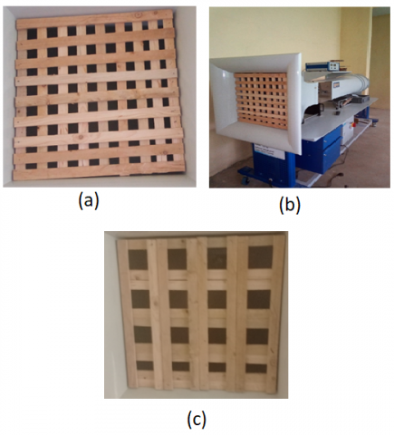
With the aim of analyzing the effects of turbulence flow on H-type vertical axis wind turbines through experimental and numerical analysis, this experimental work concentrated on the analysis of turbulence impact on vertical axis wind turbines. A vertical axis wind turbine with an H-type shape was created and tested on a small size. The wind tunnel's cross-section area is only appropriate for relatively low air velocities (0<Mach<0.2), with an overall dimension of 2890 mm×860 mm×1670 mm and a testing section of 292×292 mm in the test area. Rotating speed, power coefficient, lift and drag coefficients were investigated using wind tunnel tests as performance parameters. Experimental research was done to determine how free-stream turbulence affected the efficacy of VAWTs. The wind simulator produced turbulent flows. At the tunnel's entrance, wooden grids in three various sizes-small, medium, and large were positioned. A 0.3 m×0.3 m outlet, low-speed wind tunnel was used for the trial test. With a total length of 2.9 m, the tunnel's power section, diffuser, stilling chamber, and contract section make up the open jet type. Axial fans that were powered by electric motors under the direction of an inverter produced wind with a range of 1 to 30 m/s. In order to create turbulence inside the wind tunnel, wooden grids of the small, medium, and large grid widths were positioned at the tunnel's entrance, as shown in Figure 1. By varying the distance of the turbine from the grid location while maintaining a constant inlet velocity, the turbulence intensity was calculated. A square mesh made of square bars is the simplest method to create isotropic turbulence, according to Roach's findings [15].
Figure 1. (a) Small grids 35 mm×35 mm mesh sizes; (b) installation of turbulent grids in wind tunnel; (c) medium grids 65 mm×65 mm
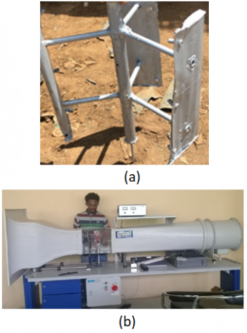
Figure 2. (a) Construction of the H-type model; (b) installation of H-type model inside the wind tunnel
The wind tunnel used was from the department of Mechanical Engineering at Debre Tabor University, Ethiopia. The wind tunnel used is aHM170 Germany product open channel subsonic type. It has dimension of 2890 mm×860 mm×1670 mm, a testing section of 292 mm×292 mm, and 292 mm (W)×292 mm (H)×460 mm (L). The speeds in the test section can reach up to 28 m/s. This allows development of stable turbulence intensity and length scale levels as seen in Figure 2.
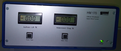
For the turbulence flow cases of 3-type square grids with different mesh size, the recording of lift and drag force can be done using digital force display instrument as seen in Figure 3 and the rotational speed using tachometer as seen in Figure 4 where wind speed was between 7-12 m/s.
Figure 3. Lift and drag force measuring instrument
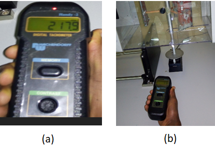
Figure 4. (a) Digital tachometer; (b) how to measure rotational speed of the turbine
The models' RPM is measured using a tachometer in various wind situations. To reflect the infrared light, a tiny piece of reflective tape was affixed to the shaft. The mirrored light is captured by a detector on the tachometer, which measures frequency variations. The VAWT model calculates the rotational speed from the frequency shift over time.
Following the experimental study, computational fluid dynamics (CFD) numerical analyses were performed using ANSYS FLUENT 15.0 software. The multi-physics ANSYS Workbench framework, which allows for the development of a workflow from CAD generation to result post-processing, was used to create the 3D CFD model. The Sliding Mesh Model was used to resolve the uneven flow. (SMM). The operating pressure of 101325 Pa and the inlet velocity of 7-12 m/s were used in the study of these 3D models.
3.1 The effact of wind velocity on the performance of the wind turbine
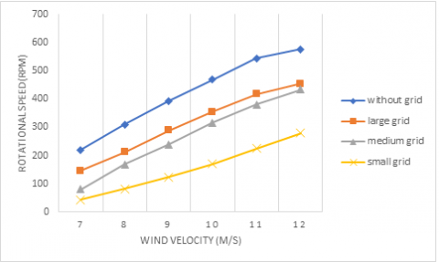
According to Figure 5, for a given freestream velocity and wind turbine rotational speed, the wind velocity (7-12 m/s) has a similar flow when compared to both without grids and with various grids (large, medium, and small). High rotational speed compared to those with squares when there are none.
This means there is a smooth flow through wind turbine and the rotation speed increases dramatically when increasing the wind speed. The large grid’s rotational speed is as low as without grid. It means the incoming wind is chaotic and there is small disturbance relative to the other grids. When compared to other grids, the small grid exhibits the worst self-starting properties under low wind speed circumstances because the incoming wind exhibits highly chaotic characteristics along with high levels of dust and storm. These severely disturbed flow fields produced very slow rotational speeds, which reduced the amount of electricity produced by the wind turbine. The rotational speed of a wind rotor at 8 m/s is 28.8% lower than it would be without a grid. In comparison to other wind turbines with grids, those without grids had the fastest rotation at greater wind speeds and the best self-starting properties in low wind speed conditions.
Figure 5. Wind velocity against rotational speed graph
3.2 Effect of turbulence on the performance wind turbine
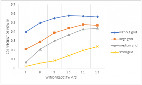
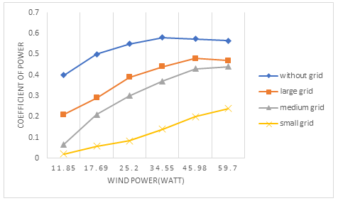
Figure 6 displays the contours with and without grid turbulence. The effects of disturbance are to blame for the low values of the power index at low tip speed ratios. As a consequence, lift is lost, and drag is increased. Furthermore, rather than being extracted from the flow, this results in power being transferred to the flow, which in turn results in low power coefficient values. The power output coefficient is increasing as the wind velocity rises, as shown in Figure 6 without a grid.
Figure 6. Wind velocity against coefficient of power graph
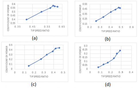
A reduction in disturbance caused by an increase in wind speed leads to an increase in power production. According to Figure 6, the power coefficient quickly drops for the small grid in the range of v<9m/s, and the rotor blades cause a high level of chaos. At low rotational speed and high air disturbance, the flow that is produced at the blade root is separated. Without the grid, the highest power coefficient is 0.58 at a speed of 10 m/s. While using a tiny grid and moving at a velocity of 12 m/s, the power coefficient is 0.24. Due to the high levels of turbulence present, the small grids exhibit a decrease in power of about 59.3% when compared to when there is no grid. At this time, the turbulence's effects are at their peak. Therefore, it can be said that the power coefficient is negatively impacted by open stream turbulence. The tip speed ratio increased as the coefficient of power and spinning speed increased. Additionally, the theory explanation in the literature that demonstrates how an increase in the tip speed ratio results in an increase in the rotational speed of the turbine supported this qualitative explanation. In every situation, greater tip-speed ratios result in the greatest efficiency. (with and without grids). Figure 7(a) shows that the power efficiency of the system without a grid increases quickly as the tip speed ratio rises before hitting its maximum value and almost tending to decrease.
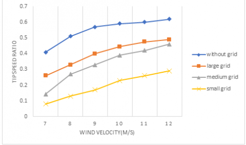
A large grid in Figure 7(b) displays the highest value of the coefficient of power at 0.48 and the λ at 0.48. A middle grid in Figure 7(c) displays power coefficients of 0.44 and λ of 0.46. In contrast, the tiny grid of Figure 7(d) displays power coefficients of 0.24 and λ of 0.29. In comparison to other various grids, the power coefficient value without a grid shows increases of 58.6%, 24.13%, and 17.24% for small grids, medium grids, and large grids, respectively. A maximum deviation of 15.25% was, however, caused by the impact of free stream turbulence on the power coefficient between the small grid and the big grid. At a low tip speed ratio of 0.08<λ<0.23, the without grid power coefficient exhibits a higher value than small grids. As can be seen in Figure 8, the coefficient of power for systems without grids is 84% greater than for systems with small grids. This results in a complete stall at the rotor blade due to flow disturbance or turbulence recovery. Additionally, the highest power coefficient without a grid is 0.58 and λ of 0.6 respectively. Without grids, the power coefficient and λ are both 0.4 and 0.41 at the speed reduction.
Figure 7. Coefficient of power curves: (a) without grid; (b) large grids; (c) medium grid; (d) small grid
The large grid shows power coefficient of 0.21 and λ of 0.26. The medium grid exhibits power coefficient of 0.068 and λ of 0.14. While the small displays power coefficient of 0.022 and λ of 0.08. For small, medium, and large grids, respectively, the power coefficient performance reveals decreases of 94.5, 83.3, and 47.5 percent. Therefore, for all grids, the turbulence effect is greater at low tip speed ratios, and the turbulence effect also grows as the grid mesh size is decreased.
Figure 8. Wind velocity against tip speed ratio graph
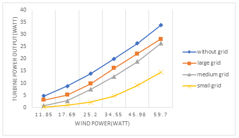
3.3 Effect of turbine power output on the performance free flow and turbulence flow
As shown in Figure 9, the total power is inversely proportional to the coefficient of performance. This demonstrates that increasing the performance of wind turbines while increasing the generated electricity from wind turbines with or without grids. Small grid reduced the production of power which occurred at 7 m/s high turbulence. There is disturbance of flow which stall the effect on rotational blade. The rotational speed is very low at similar manner while the output power and power coefficent also reduced. Figure 10 shows that at 8 m/s, Pw is 17.69 and Pt is 8.845 for without grids. Pw is 17.69 and Pt is 5.2 for large grids. While Pw is 17.69 and Pt is 2.83 for medium grid. Finally, Pw is 17.69 and Pt is 1.04 for small grid. The turbine power conversion has 40%, 21%, 6.8% and 2.2% for without grid, large grid, medium grid and small grid respectively. The average turbine power conversion is 52.8%, 38%, 30.3% and 2.4% for without grid, large, medium and small grids respectively.
Figure 9. Wind power against coefficient of power graph
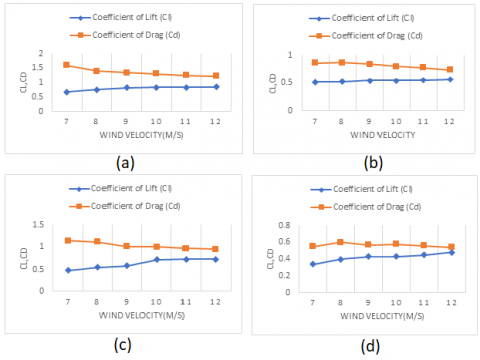
3.4 Lift and drag coefficient with variable wind velocity
As shown in Figure 11, the graphs for all cases with and without grids almost get constant level. The coefficient of lift increases as the wind velocity increases. However, the coefficient of drag decreases as the wind velocity decreases. Figure 11 shows that the coefficient of lift increases and coefficient of drag decrease dramatically until the constant level relatively too with grids.
Figure 10. Wind power against turbine power output graph
Figure 11. Coefficient of lift and drag: (a) without grid; (b) large grid sizes; (c) medium grid sizes; (d) small grid sizes
Figure 12. Turbulence intensity against tip speed ratio: (a) without grids; (b) large grids; (c) medium grids; (d) small grids graph
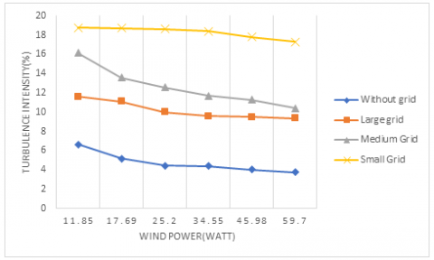
3.5 Effect of turbulence intensity on the power performance
Strong disturbance in natural wind results in dynamic stalling of vertical axis wind turbines (VAWTs), which can significantly alter power coefficient performance [16-21]. Therefore, in the VAWT design process, it is essential to comprehend how turbulence intensity affects the power performance traits. The turbulence grid was used to create turbulence strength. In Figure 12(d), small grid shows maximum turbulence intensity TI of 18.74%, and λ of 0.08. In Figure 12(c), medium grid displays maximum turbulence intensity TI of 16.14% and λ of 0.144. In Figure 12(b), large grid shows maximum turbulence intensity TI of 11.6% and λ of 0.26. While in Figure 12(a), without grids shows maximum turbulence intensity TI of 6.65% and λ of 0.41.
Turbulence intensity values indicate that the small grid has greater percentages of 64.5%, 38.1%, and 12.6% than the large grid, medium grid, and without grid, respectively. Additionally, with a velocity of 7 m/s, the power coefficient reveals reductions of 94.5%, 89.5%, and 67.4% in comparison to no grid, large grid, and medium grid, respectively. There is inverse relationship between the turbulence intensity and the coefficient of power. Figure 13 shows that turbulence intensity increases when there is increase in grid mesh sizes. Small grid size has higher turbulence intensity as compared to others because of blockage area of the incoming wind. As seen in Figure 12, turbulence intensity decreases when there is increase in the tip speed ratio for all cases with and without grids.
Figure 13. Turbulence intensity against wind power
3.6 Numerical results
3.6.1 Analysis coefficient of power in ANSYS FLUENT
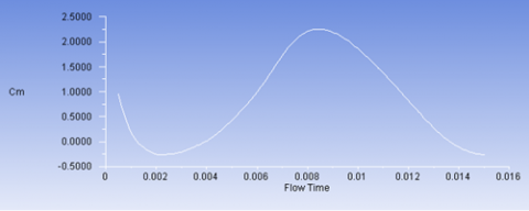
Following the experimental study, computational fluid dynamics (CFD) numerical analyses were performed using ANSYS FLUENT 15.0 software. The multi-physics ANSYS Workbench framework, which allows for the development of a workflow from CAD generation to result post-processing, was used to create the 3D CFD model. The Sliding Mesh Model was used to resolve the uneven flow. (SMM). The operating pressure of 101325 Pa and the inlet velocity of 7-12 m/s were used in the study of these 3D models. Figures 14-17 display the findings of each model iteration's moment of coefficients as determined by FLUENT.
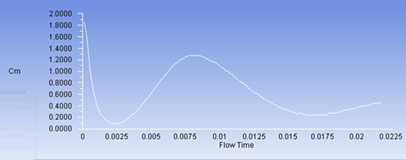
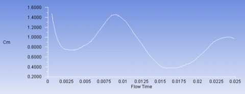
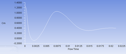
The plots in Figures 14 to 17 oscillate as a result of the blades' rotation. Every maximum and lowest happened when the airfoils were in alignment with one another. In order to analyze the FLUENT findings, text files were opened in Excel. In Excel, the average value of each line was calculated in order to determine the precise value of the rotor's power coefficient under various operating circumstances. This procedure was performed for each gris and velocity in order to examine the FLUENT outcomes. Although power coefficient values for the rotor must also be derived, moment coefficient values were acquired from FLUENT. In order to obtain the values of the power coefficient as indicated by Eq. (1), the tip speed ratio was multiplied by the average value of the moment coefficient:
$\mathrm{Cp}=\mathrm{Ct} \times \lambda$ (1)
The same procedure was followed for different velocity and grid sizes in order to obtain all the values of power coefficient Cp and moment coefficient as shown in Table 1.
Figure 14. Coefficient of power curve without grid at 7m/s wind velocity
Figure 15. Coefficient of power curve large grid sizes grid at 7m/s wind velocity
Figure 16. Coefficient of power curve medium grid sizes grid at 7m/s wind velocity
Figure 17. Coefficient of power curve small grid sizes at 7m/s wind velocity
3.7 Validation of CFD simulation
Figure 18 compares the experimental data of the power coefficient at various grids with the CFD findings. In order to completely comprehend the flow structures around the model turbine, computational predictions were made. Figure 18 illustrates how the simulation results and the experimental data looked to be relatively well matched. There are, however, a few minuscule variations found.
Table 1. Average value of coefficient of moment and coefficient of power
|
|
Without Grid |
Large Grid |
Medium Grid |
Small Grids |
||||
|
Wind Velocity |
Cmaverage |
Cpaverage |
Cmaverage |
Cpaverage |
Cmaverage |
Cpaverage |
Cmverage |
Cpaverage |
|
7 |
0.94 |
0.39 |
0.91 |
0.24 |
0.7 |
0.1 |
0.61 |
0.048 |
|
8 |
0.92 |
0.46 |
0.88 |
0.29 |
0.73 |
0.2 |
0.64 |
0.082 |
|
9 |
0.91 |
0.52 |
0.86 |
0.35 |
0.75 |
0.26 |
0.66 |
0.11 |
|
10 |
0.95 |
0.56 |
0.89 |
0.4 |
0.78 |
0.31 |
0.69 |
0.16 |
|
11 |
0.97 |
0.58 |
0.93 |
0.45 |
0.82 |
0.38 |
0.71 |
0.19 |
|
12 |
0.98 |
0.59 |
0.95 |
0.47 |
0.85 |
0.4 |
0.73 |
0.22 |
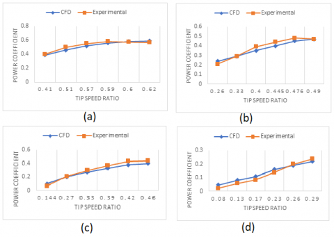
Figure 18. Comparison of coefficient of power of experimental and numerical results (a) without grids (b) large grid sizes (c) medium grid sizes (d) small grid sizes
From Figure 18(a), the experimental data coefficient of power was slightly higher than that of CFD simulations at 0.41<λ<0.6. It can also be seen that the experimental result was very close to the numerical results. Minimum deviation of 1.8% occurs at value of λ at 0.6 and maximum deviation of 8.5% at value of λ at 0.51. The averaged relative deviation is 4.83%. Moreover, as seen in Figure 18(b), the average deviation of large grids was 6%. Moreover, the purpose of applying numerical simulation in comparing to experimental result is for comparative analysis of aerodynamic performance. Figure 18(c) shows that maximum deviation occurred at value of λ at 0.144 and this corresponds to 13% maximum deviation and minimum deviation occurs at the value of λ at 0.27 and also corresponds to 5% minimum deviation. The averaged relative deviation was 5.3%. At low tip speed ratio, the CFD results were higher, but at high tip speed ratio, it was inverse of the experimental results because the experimental results were lower as seen in Figure 18(d). The simulation findings and the experimental data seemed to match up relatively well. Despite the small deviations that were noticed, the maximum deviation was 16%, and the minimum deviation was 4.5%. There was an 8% average variation.
Turbulence intensity values indicate that the small grid has greater percentages of 64.5%, 38.1%, and 12.6% than the large grid, medium grid, and without grid, respectively. Additionally, with a velocity of 7 m/s, the power coefficient reveals reductions of 94.5%, 89.5%, and 67.4% in comparison to no grid, large grid, and medium grid, respectively. The coefficient of power and the strength of the turbulence are inversely related.
Due to the high levels of turbulence present at this point, the small grids exhibit a decrease in power of about 59.3% when compared to those without grids. Therefore, it can be said that the power coefficient is negatively impacted by open stream turbulence.
Maximum turbulence intensity (TI) on the small grid is 18.74%, and the λ value is 0.08. The medium grid shows a highest TI of 16.14% and a λ of 0.144 for the turbulence intensity. The large grid displays a highest TI of 11.6% and a λ of 0.26. Without grids, the highest turbulence intensity is 6.65% and the coefficient of turbulence is 0.41. Turbulence intensity values indicate that the small grid has greater percentages of 64.5%, 38.1%, and 12.6% than the large grid, medium grid, and without grid, respectively. In addition, the power coefficient is lower with a velocity of 7 m/s than it is with no grid, a big grid, and a medium grid, respectively, by 94.5 percent, 89.5 percent, and 67.4 percent.
[1] Talavera, M., Shu, F. (2017). Experimental study of turbulence intensity influence on wind turbine performance and wake recovery in a low-speed wind tunnel. Renewable Energy, 109: 363-371. https://doi.org/10.1016/j.renene.2017.03.034
[2] Wong, K.H., Chong, W.T., Sukiman, N.L., Poh, S.C., Shiah, Y.C., Wang, C.T. (2017). Performance enhancements on vertical axis wind turbines using flow augmentation systems: A review. Renewable and Sustainable Energy Reviews, 73: 904-921. https://doi.org/10.1016/j.rser.2017.01.160
[3] Loganathan, B., Mustary, I., Chowdhury, H., Alam, F. (2017). Effect of turbulence on a Savonius type micro wind turbine. Energy Procedia, 110: 549-554. https://doi.org/10.1016/j.egypro.2017.03.183
[4] Pagnini, L.C., Burlando, M., Repetto, M.P. (2015). Experimental power curve of small-size wind turbines in turbulent urban environment. Applied Energy, 154: 112-121. https://doi.org/10.1016/j.apenergy.2015.04.117
[5] Siddiqui, M.S., Rasheed, A., Kvamsdal, T., Tabib, M. (2015). Effect of turbulence intensity on the performance of an offshore vertical axis wind turbine. Energy Procedia, 80: 312-320. https://doi.org/10.1016/j.egypro.2015.11.435
[6] Devinant, P., Laverne, T., Hureau, J. (2002). Experimental study of wind-turbine airfoil aerodynamics in high turbulence. Journal of Wind Engineering and Industrial Aerodynamics, 90(6): 689-707. https://doi.org/10.1016/S0167-6105(02)00162-9
[7] Kamada, Y., Maeda, T., Murata, J., Yusuke, N. (2016). Effect of turbulence on power performance of a horizontal axis wind turbine in yawed and no-yawed flow conditions. Energy, 109: 703-711. https://doi.org/10.1016/j.energy.2016.05.078
[8] Lubitz, W.D. (2014). Impact of ambient turbulence on performance of a small wind turbine. Renewable Energy, 61: 69-73. https://doi.org/10.1016/j.renene.2012.08.015
[9] Wekesa, D.W., Wang, C., Wei, Y., Zhu, W. (2016). Experimental and numerical study of turbulence effect on aerodynamic performance of a small-scale vertical axis wind turbine. Journal of Wind Engineering and Industrial Aerodynamics, 157: 1-14. https://doi.org/10.1016/j.jweia.2016.07.018
[10] Chu, C.R., Chiang, P.H. (2014). Turbulence effects on the wake flow and power production of a horizontal-axis wind turbine. Journal of Wind Engineering and Industrial Aerodynamics, 124: 82-89. https://doi.org/10.1016/j.jweia.2013.11.001
[11] Hamada, K., Smith, T., Durrani, N., Qin, N., Howell, R. (2008). Unsteady flow simulation and dynamic stall around vertical axis wind turbine blades. In 46th AIAA Aerospace Sciences Meeting and Exhibit, p. 1319. https://doi.org/10.2514/6.2008-1319
[12] Anbaei, S., Ziaei-Rad, M., Aryaei, A., Afshari, E. (2018). Numerical simulation of turbulent flow through a three-blade vertical axis wind turbine. 16th International Conference on Clean Energy (ICCE-2018) 9-11 May 2018, Famagusta, N. Cyprus.
[13] Karbasian, H.R., Esfahani, J.A., Barati, E. (2016). Effect of acceleration on dynamic stall of airfoil in unsteady operating conditions. Wind Energy, 19(1): 17-33. https://doi.org/10.1002/we.1818
[14] Howell, R., Qin, N., Edwards, J., Durrani, N. (2010). Wind tunnel and numerical study of a small vertical axis wind turbine. Renewable Energy, 35(2): 412-422. https://doi.org/10.1016/j.renene.2009.07.025
[15] Roach, P.E. (1987). The generation of nearly isotropic turbulence by means of grids. International Journal of Heat and Fluid Flow, 8(2): 82-92. https://doi.org/10.1016/0142-727X(87)90001-4
[16] Ahmadi-Baloutaki, M., Carriveau, R., Ting, D.S.K. (2015). Performance of a vertical axis wind turbine in grid generated turbulence. Sustainable Energy Technologies and Assessments, 11: 178-185. https://doi.org/10.1016/j.seta.2014.12.007
[17] Möllerström, E., Ottermo, F., Goude, A., Eriksson, S., Hylander, J., Bernhoff, H. (2016). Turbulence influence on wind energy extraction for a medium size vertical axis wind turbine. Wind Energy, 19(11): 1963-1973. https://doi.org/10.1002/we.1962
[18] Al-Abadi, A., Seok, J., Hartl, M. (2014). Experimental investigations of the turbulence impact on the performance of the HAWT. In 10th PhD Seminar on Wind Energy, pp. 7-11.
[19] Cao, L., Wang, H., Ji, Y., Wang, Z., Yuan, W. (2012). Analysis on the influence of rotational speed on aerodynamic performance of vertical axis wind turbine. Procedia Engineering, 31(1): 245-250. https://doi.org/10.1016/j.proeng.2012.01.1019
[20] Shahzad, A., Asim, T., Mishra, R., Paris, A. (2013). Performance of a vertical axis wind turbine under accelerating and decelerating flows. Procedia CIRP, 11: 311-316. https://doi.org/10.1016/j.procir.2013.07.006
[21] Kooiman, S.J, Tullis, S.W. (2010). Response of a vertical axis wind turbine to time varying wind conditions found within the urban environment. Wind Engineering, 34(4): 389-401. https://doi.org/10.1260/0309-524X.34.4.389