Feraoun Ali*![]() | Merouane Habib
| Merouane Habib![]() | Sahnoun Rachid
| Sahnoun Rachid![]()
© 2023 IIETA. This article is published by IIETA and is licensed under the CC BY 4.0 license (http://creativecommons.org/licenses/by/4.0/).
OPEN ACCESS
This research undertakes a numerical investigation of an axisymmetric double-jet semi-confined annular flow produced by a burner. The endeavor aims to thoroughly decipher the behavior of these turbulent flows within a double annular jet, with a focus on characterizing the mixing and recirculation regions. Analyses of the annular jet were conducted for three distinct Reynolds numbers (6683, 8874, and 11065). Numerical simulations were performed using a computational fluid dynamics (CFD) calculation code, employing two turbulence models-k-epsilon and SST k-ω. The governing differential equations, discretized for the flow, were solved via the finite volume method, utilizing the semi-implicit method algorithm for pressure-linked equations. Findings revealed the existence of three recirculation zones separated by the annular jets. The first, a minute zone, is situated between the two annular jets. The second, a medium-sized zone, resides just behind the nozzle near the injection axis, below the primary jet. The third, a large zone, is positioned near the upper wall of the combustion chamber. It was observed that the size of the initial small recirculation zone exhibited negligible variation with changes in the Reynolds number. However, the second medium-sized zone experienced notable alterations with the Reynolds number. The third large zone generated an extensive toroidal vortex at higher Reynolds numbers. These recirculation zones offer potential for control to optimize fuel-air mixing, aiming to achieve near-perfect combustion while minimizing pollutant emissions. The numerical simulation results generally exhibited strong agreement with experimental findings.
annular jets, double jet annular flow, burner jet, turbulent flow
Turbulent flows within annular jets are commonly utilized across numerous energy systems, including gas turbines, industrial furnaces, combustors, and burners. Investigations into these flows yield invaluable insights into the fluid dynamics within the combustion chambers of these systems. This knowledge can subsequently be harnessed to enhance system performance, reduce fuel consumption, and minimize the emission of pollutants such as NOx and CO2. Research into annular double-jet flows, however, remains relatively scarce, necessitating additional experimental and numerical studies to fully comprehend the flow field behavior and associated combustion processes in burners.
Past research has predominantly focused on annular jets with a single jet. Works by Del Taglia et al. [1], Danlos et al. [2], Zhang and Vanierschot [3], Ryzhenkov et al. [4], Vanierschot et al. [5], Yang et al. [6], Sadr et al. [7], and Trávnı́ček and Tesař [8] serve as key examples. Conversely, studies on flows with double annular jets have been less frequent, with notable contributions made by Vucinic and Hazarika [9], Broeckhoven et al. [10], and Huang and Tsai [11].
A noteworthy investigation into a double annular jet was conducted by Schmitt et al. [12] using 2D Laser Doppler Velocimetry (LDV) measurements. Their findings confirmed good axisymmetricity of the measurements. The double annular geometry was found to generate a complex flow, characterized by recirculation regions, multiple toroidal vortices, and the presence of stagnation points and lines. Comprehensive descriptions of the first and second moments of the velocity field on a detailed experimental grid have been acquired, forming a valuable database for comparison with turbulence models.
Hazarika et al. [13] conducted an experimental study on the flow within a confined annular double jet. Employing particle image velocimetry and laser Doppler velocimetry, flow visualization was carried out across a spectrum of Reynolds numbers, spanning from laminar to turbulent regimes. It was observed that the time-averaged velocity field maintained a consistent topology within the examined range of Reynolds numbers, with variations in the extent of different regions correlating with changes in the Reynolds number. The recirculation zones situated behind the bluff bodies exhibited an increase with rising Reynolds numbers, peaking before gradually converging to an asymptotic value.
Geerts et al. [14] undertook the validation of various turbulence models, comparing them with experimental results for the complex turbulent flow of an axisymmetric confined annular double jet. The structural analysis included axial and radial velocities as well as turbulent kinetic energy profiles. These were calculated using the algebraic model (Baldwin-Lomax), the one-equation model (Launder Sharma), and different k- turbulence models (Chien, Spalart Allmaras, and Yang Shih). It was noted that all models appeared to accurately predict the global flow characteristics, although the k-Yang Shih turbulence model demonstrated superior tracking of fine-scale flow properties.
Murugan et al. [15] delved into the influence of annular pulsation on the flow characteristics and mixing properties of low Reynolds number concentric twin jets. The annular pulsation was initiated using a solenoid valve, with the jet spread widths computed via a binary edge detection technique. Through the application of Particle Image Velocimetry (PIV), time-averaged velocity vectors, streamline patterns, turbulence intensity distributions, and vorticity contours were analyzed. It was observed that the annular pulsations led to a significant increase in turbulence intensity within the flow field, attributed to the axial elongation of the recirculation region. The elongation of this zone, coupled with intermittent stagnation points, facilitated the efficient dispersion of the central jet within the annular flow. A radial dispersion enhancement index indicated that the mixing capability between the jets could be improved by up to 80% within the recirculation region through the application of annular pulsations.
While notable research has been conducted on simple annular jets, studies focusing specifically on double annular jets remain relatively scarce. To address this gap, the current work aims to conduct an in-depth study of double annular jets across varying Reynolds numbers.
The focal point of this investigation is a numerical study of an axisymmetric semi-confined annular double jet, generated by a burner, at different Reynolds numbers (6683, 8874, and 11065). Emphasis is placed on understanding the behavior of turbulent flows within annular jets, with the aim of effectively controlling the size of the initial recirculation zone. This control is crucial to promoting reactive mixing and stabilizing the flame within combustion chambers. The modeling process utilizes a Computational Fluid Dynamics (CFD) calculation code, employing two turbulence models, k-epsilon, and SST k-ω. The discretized differential equations governing the flow are resolved using the finite volume method and the semi-implicit method for pressure-linked equations. The numerical results obtained from the simulation are then compared with experimental findings.
For the modeling of the annular flow we chose the RANS approach method (RANS for Reynolds Average Navier-stokes because this method is more widely developed and requires lower computational cost. The turbulence models used are k-epsilon and SST k-ω. The major disadvantage of these models is that they are very limited for the anisotropic turbulent flows.
2.1 The k-epsilon model
The k-epsilon model has many advantages: it is a relatively simple model, requiring only two additional equations (k and ε), available in almost all codes, the model has great robustness which allows in particular to tackle complex physical problems. This model is proposed by Launder et al. [16] which is based on the Boussinesq approximation.
$\tau_{i j}=\mu_t\left(\frac{\partial \bar{u}_i}{\partial x_j}+\frac{\partial \bar{u}_j}{\partial x_i}\right)-\frac{2}{3} \mu_t \frac{\partial \bar{u}_k}{\partial x_k} \delta_{i j}-\frac{2}{3} \rho k$ (1)
The turbulent viscosity is determined by:
$\mu_t=\rho C_\mu \frac{k^2}{\varepsilon}$ (2)
With ε is the dissipation rate given by:
$\varepsilon=\frac{\mu_t}{\rho}\left(\overline{\frac{\partial u_i}{\partial u_j} \frac{\partial u_i}{\partial u_j}}\right)$ (3)
The two additional equations are:
$\rho u \nabla k=\nabla\left[\left(\mu+\frac{\mu_t}{\sigma_k}\right) \nabla k\right]+G_k-\rho \mathcal{E}+S_k$ (4)
$\rho u \nabla \varepsilon=\nabla\left[\left(\mu+\frac{\mu_t}{\sigma_{\varepsilon}}\right) \nabla \varepsilon\right]+C_{\varepsilon 1} \frac{\varepsilon}{k} G_k-C_{\varepsilon 2} \rho \frac{\varepsilon^2}{k}+S_{\varepsilon}$ (5)
where, Gk is the turbulence kinetic energy due to the mean velocity, σk and σε are the turbulent Prandtl numbers for k and ε respectively. Cε1, Cε2 are the constants, the coefficients are given in Table 1.
Table 1. Constants for the standard k-ε model
|
Cμ |
Cε1 |
Cε2 |
σk |
σε |
|
0.09 |
1.44 |
1.92 |
1.0 |
1.3 |
2.2 The SST K- ω model
The Shear Stress Transport k-ω model, proposed by Menter [17] in 1994, is a hybrid model using different turbulence models for the near-wall region and in the rest of the flow.
The turbulent viscosity is given by:
$\mu_t=\frac{\rho a_1 k}{\max \left(a_1 \omega, S F_2\right)}$ (6)
with
$F_2=\tanh \left[\left[\max \left(\frac{2 \sqrt{k}}{\beta^* \omega y}, \frac{500 v}{y^2 \omega}\right)\right]^2\right]$ (7)
where, S is magnitude of the mean velocity gradients
$S=\sqrt{2 S_{i j} S_{i j}}$ (8)
The two additional equations are:
$\rho u \nabla k=P_k-\rho \beta^* k \omega+\nabla\left(\left(\mu+\sigma_k \mu_t\right) \nabla k\right)$ (9)
$\begin{aligned} & \rho u \nabla \omega=\rho \alpha S^2-\rho \beta \omega^2+\nabla\left(\left(\mu+\sigma_k \mu_t\right) \nabla \varepsilon\right) \\ & +2\left(1-F_1\right) \sigma_{\omega 2} \frac{\rho}{\omega} \nabla \omega \nabla k\end{aligned}$ (10)
where,
$P_k=\min \left[\tau_{i j} \frac{\partial U_i}{\partial x_j}, 10 \beta^* k \omega\right]$ (11)
$F_1=\tanh \left\{\min \left[\max \left(\frac{\sqrt{k}}{\beta^* \omega y}, \frac{500 v}{y^2 \omega}\right), \frac{4 \sigma_{\omega 2} k}{C D_{k \omega} y^2}\right]^4\right\}$ (12)
$C D_{k \omega}=\max \left(2 \rho \sigma_{\omega 2} \frac{1}{\omega} \frac{\partial k}{\partial x_i} \frac{\partial \omega}{\partial x_i}, 10^{-10}\right)$ (13)
where, y is the distance to the next surface and CDkω is the positive portion of the cross-diffusion term.
The SST k-ω constants are given in Table 2.
Table 2. Constants for the SST k-ω model
|
β* |
β2 |
a1 |
σk,1 |
σω,1 |
σk,2 |
σω,2 |
|
|
0.0828 |
0.31 |
0.85 |
0.5 |
1.0 |
0.856 |
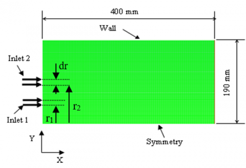
The geometry consists of two rings of outer radius r1=50.5 mm and r2=78 mm with thickness dr=8 mm (Table 3). The length of the geometry is determined only from the outlet of the burner to the end of the combustion chamber which is shown in Figure 1.
Table 3. Double annular jets parameter
|
Parameter |
Description |
Dimension |
|
r1 |
radius of the primary jet |
50.5 mm |
|
r2 |
radius of the secondary jet |
78.0 mm |
|
dr |
width of annular jets |
8.0 mm |
|
rc |
combustion chamber radius |
190 mm |
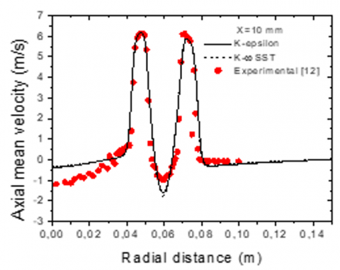
The mesh test sensitivity was chosen by testing two different meshes with different quadrilateral cell nodes and elements. The first type of mesh (grid 1) is constituted by 9792 nodes and 9550 quadrilateral cells with 18859 interior faces. The second mesh (grid 2) has 19392 nodes and 19100 quadrilateral cells with 37909 interior faces. The test of the two meshes is carried out for the inlet axial mean velocity U1=6.3 m/s and U2=6.1 m/s in the position X=10 mm (Figure 2). The results obtained for the two mesh tests are similar and agree very well with the experimental data.
Figure 1. Computational combustion chamber
Figure 2. Mesh test sensitivity
The boundary conditions are very important to obtain an accurate solution with fast convergence. The boundary conditions are determined for four borders based on experimental data given by Schmitt et al. [12]:
At the inlet of the two annular jets (inlet 1, inlet 2) the axial velocity U1=6.3 m/s and U2=6.1 are imposed for the primary and the secondary annular jet, the Reynolds number is calculated for different axial velocity in the secondary annular jet (U2=6.1, 8.1 and 10.1m/s) by:
$\operatorname{Re}_{D h}=\frac{U_2 2 d r \rho_{\text {air }}}{\mu_{\text {air }}}$ (14)
where,
ReDh: is the hydraulic diameter in the secondary annular jet.
μair: is the air dynamic viscosity, μair=1.789 e-5 kg/m.s.
ρair: is the air density, ρair=1,225 kg/m3.
The primary axial velocity is maintained constant U1=6.3 m/s.
At the outlet of the combustion chamber the absolute pressure is imposed.
At the wall boundary condition the no-slip condition is applied with u=v=0 and k=ε=0.
u and v are the axial and radial velocity respectively.
k and ε are the turbulent kinetic energy and the dissipation rate respectively.
In the axial of the combustion chamber the symmetry condition is applied $\frac{\partial u}{\partial y}=\frac{\partial v}{\partial y}=0$ and $\frac{\partial P}{\partial y}=0$.
We present in this party a numerical study of an axisymmetric semi-confined annular double-jet flow consisting two coaxial annular jets. The flow is generated by a burner for different Reynolds numbers (6683, 8874 and 11065). The flow is studied without combustion to understanding the behavior of the recirculation zone, instabilities and shear layers. The modeling is carried out using a CFD calculation code by the use of two turbulence models k-epsilon and SST k-ω.
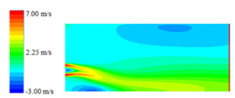
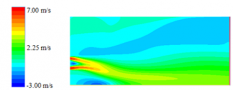
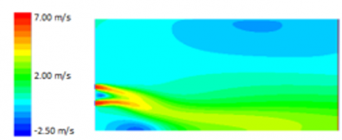
Figures 3 and 4 present the contour of the mean axial velocity obtained by numerical simulation by the two models of turbulence k-epsilon and SST k-ω. We observe in these figures the presence of three recirculation zones with different seize, small, medium and large. The first small zone is located between the two annular jets; the second medium-sized is located just near the injection of the flow in the combustion chamber, which plays a very important role during fuel injection (air+fuel). This area creates a very large depression which gives negative velocity; this depression generates a vortex movement which allows the gaseous fuel to mix well with the air. We also note the presence of a third zone of very large size located just in the upper part of the combustion chamber, this zone does not have much influence on the mixture combustion. The recirculation zones are characterized by a stagnation point, a vortex center point, and a length.
The numerical results obtained by the two models are very similar and the annular jet is characterized by a principal recirculation zone near the jet axis.
Figure 3. Contours of the mean axial velocity (k-ε model)
Figure 4. Contours of the mean axial velocity (SST k-ω model)
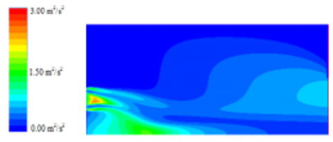
Figure 5. Contours of the turbulent kinetic energy (k-ε model)
Figure 6. Contours of the turbulent kinetic energy (SST k-ω)
Figures 5 and 6 present the turbulent kinetic energy contour obtained by numerical simulation with the two models k-epsilon and SST k-ω. These figures illustrate a strong concentration of the turbulent kinetic energy localized between the two annular jets and in the recirculation zone which is just near the injection. It is also observed that the turbulent kinetic energy is important in the inner and outer shear layers created by the two annular jets, this intensity of turbulent kinetic energy decreases gradually when the flow is established and became stable, the creation of energy turbulent kinetics in the combustion zone plays a very important role in promoting reactive mixing.
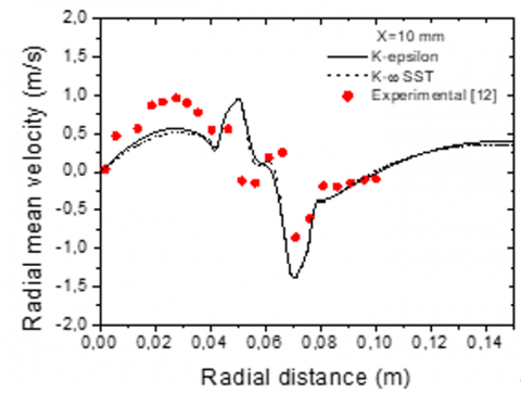
Figure 7. Axial mean velocity at axial position X=10 mm
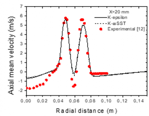
Figure 8. Axial mean velocity at axial position X=20 mm
We can conclude in these figures that the turbulent kinetic energy is well concentrated between the two annular jets and the recirculation zone which is located just near the injection.
Figure 7 presents the profile of the mean axial velocity varies according to the radial distance obtained by numerical simulation with the two models k-epsilon and SST k-ω at the axial distance X=10 mm compared with the experimental obtained by Schmitt et al. [12]. We observe in this figure two peaks of the axial velocity with maximum magnitude of 6.3 m/s generated by the two annular jets of the flow. We also observe a minimum peak of -1.6 m/s; this minimum velocity is caused by the recirculation zone between the two annular jets. The results obtained by numerical simulation are in good agreement with the experimental with an underestimation near the symmetry axis. This underestimation is mainly due to the initial conditions, the configuration of the geometry in two dimensions and the models of turbulence.
Figure 8 presents the profile of the mean axial velocity varies according to the radial distance obtained by numerical simulation by with the two models k-epsilon and SST k-ω at the axial distance X=20 mm. We observe in this figure two same peaks of mean axial velocity with maximum lower magnitudes than of the distance X=10 mm, the two maximum peaks have values of 5.8 and 5.5 m/s respectively. The minimum velocity peak is -0.42 for the simulation and -1.58 m/s for the experimental case. The results obtained by numerical simulation are in good agreement with the experimental. The numerical results obtained show that the peaks of the mean axial velocity decrease with the axial distance.
Figure 9 presents the axial velocity profile varies according to the radial distance obtained by numerical simulation with the two models k-epsilon and SST k-ω at the axial distance X=40 mm. We notice in this figure the damping of the two peaks of velocity with different and lower magnitudes compared to the previous axial position, the first magnitude has a value of 5.1 m/s and the second magnitude has a value of 4.1 m /s. A positive minimum velocity peak of 2.5 m/s is also observed, which explains the disappearance of the recirculation zone between the two annular jets. The results obtained by numerical simulation are in good agreement with the experimental one.
Figure 10 presents the radial mean velocity profile varies according to the radial distance obtained by numerical simulation by the two k-epsilon and SST k-ω models at the axial distance X=10 mm. We can see in this figure the existence of two peaks of maximum and minimum radial mean velocity almost opposite to each other with a maximum peak of a value close to 0.95 m/s and a minimum peak with a value of -1.4 m/s, and then the radial mean velocity is established to reach values close to zero. The results obtained by numerical simulation are sensibly close to the experimental data. The distinction between the opposite radial mean velocity peaks is due to the primary and secondary jets and the interior and exterior shear layers.
Figure 9. Axial mean velocity at axial position X=40 mm
Figure 10. Radial mean velocity at axial position X=10 mm
Figure 11 presents the radial mean velocity profile varies according to the radial distance obtained by numerical simulation by the two k-epsilon and SST k-ω models at the axial distance X=20 mm. We also observe in this figure the existence of two peaks of maximum and minimum radial velocity peaks. The maximum peak has a value of 0.89 m/s and the minimum peak has a value of -1.79 m/s. The radial mean velocity profile preserved the same evolution as the profile in Figure 10 with slightly different values. The results obtained by numerical simulation are approximately in good agreement with the experimental data.
Figure 12 presents the radial velocity profile varies according to the radial distance obtained by numerical simulation by the two models k-epsilon and SST k-ω at the axial distance X=40 mm. We observe in this figure a disappearance of the maximum positive peak of the radial velocity which takes a very low negative magnetic value of -0.4 m/s, we also observe the appearance of two minimal peaks with different values and which are significantly low compared to the previous axial position, the first quantity has a value of -0.61 m/s and the second magnitude has a value of -1.1 m/s. The velocity is then established to reach values close to zero. The results obtained by numerical simulation are approximately in good agreement with the experimental data.
Figure 11. Radial mean velocity at axial position X=10 mm
Figure 12. Radial mean velocity at axial position X=40 mm
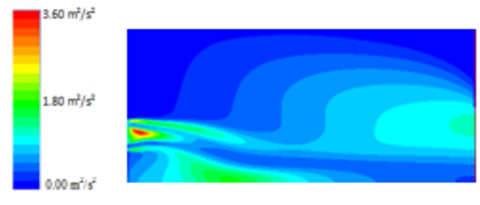
Figures 13, 14 and 15 show the results of the mean axial velocity contours obtained by the k-epsilon model for different Reynolds numbers (6683, 8874 and 11065). We observe in these figures the presence of three recirculation zones separated by the annular jets, the first zone of very small size is located between the two annular jets near the inlet condition, the second zone of medium size is located just behind the nozzle near the axis injection below the primary jet, the third large zone is located above the secondary jet near the upper wall of the combustion chamber. The first very small zone recirculation is formed by the different velocities that exist between the two annular jets and the stagnant air located between these two annular jets. We also observe that even after the variation of the Reynolds number, the size of the small recirculation zone changes almost only slightly. For the second medium-sized zone, the size of this zone changes considerably depending on the variation of the Reynolds number. For the third large zone, we observe that for a higher Reynolds number the secondary annular jet generates a very large toroidal vortex between the combustion chamber wall and the secondary jet. With these observations and numerical findings we can note that it is therefore important to carefully control the size of the recirculation zone which is located just next to the injection in order to properly mix the fuel with the air in this zone to produce the most perfect combustion and minimize pollution emissions.
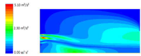
Figures 16, 17 and 18 present the results of the turbulent kinetic energy contours calculated by the k-epsilon model for different Reynolds numbers (6683, 8874 and 11065). The turbulent kinetic energy depends on the fluctuating velocity components $k=1 / 2\left(\overline{u^{\prime 2}}+\overline{v^{\prime 2}}\right)$ , these fluctuating velocity components also depend on the velocity of the annular jets. We observe in these figures that the turbulent kinetic energy is mainly concentrated in the recirculation zones and the internal and external shear layers in the edges of the primary and secondary annular jets; this turbulent kinetic energy has maximum values at the center of the small recirculation zone which is located between the two annular jets and which is limited by the size of this recirculation zone and which increases as a function of the Reynolds number. We also notice that the turbulent kinetic energy has significant values at the level of the medium-sized recirculation zone which is located just near the injection and its value also depends on the Reynolds number. We also notice that this zone was moved a little away from the proximity of the injection in the axial direction near the axis of symmetry when the Reynolds number increased. We also observe that the turbulent kinetic energy is quite significant in the large zone which develops considerably when the Reynolds number is increased. These observations can help us to know the area’s most stressed at turbulent intensities.
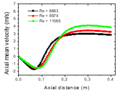
Figure 19 presents the mean axial velocity profile obtained by the k-epsilon model which varies with axial distance for different Reynolds numbers (6683, 8874 and 11065). The velocity profile can be divided into three distinct parts. The first part where the velocity profiles are negative, this negative velocity is created by the recirculation zone of medium size located just near the injection and below the primary jet and which is characterized by a length and a stagnation point, the negative zone presents minimum velocity values U=-1.7 m/s at the axial distance X=0.075 m. the second part is located between the stagnation point and the flow attachment point which presents velocity profiles with ascending allure. The third part presents the fully developed flow where the flow becomes well established. We can note that these curves are characterized by two essential parameters, the length of the recirculation zone and the stagnation point. We observe in this figure that there is a certain difference between the velocity profiles and which depends on the Reynolds number. This difference is well observed in the length of the recirculation zone and the stagnation point; for the case where the Reynolds number Re=6683 the stagnation point is located at X=0.1 m; for Re=8874 the stagnation point is located at X=0.12 m and for Re=11065 the stagnation point is located at X=0.13 m.
Figure 13. Mean axial velocity contours for Re=6683
Figure 14. Mean axial velocity contours for Re=8874
Figure 15. Mean axial velocity contours for Re=11065
Figure 16. Contours of turbulent kinetic energy for Re=6683
Figure 17. Contours of turbulent kinetic energy for Re=8874
Figure 18. Contours of turbulent kinetic energy for Re=11065
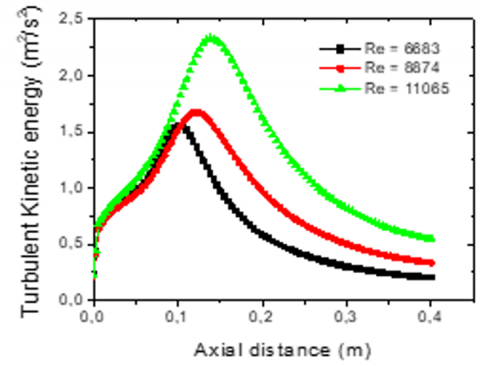
Figure 20 shows the turbulent kinetic energy profile obtained by the k-epsilon model which varies with the axial distance for different Reynolds numbers (6683, 8874 and 11065). It is observed in these figures that the profiles of the turbulent kinetic energy increase in a quasi-linear manner in the medium-sized recirculation zone to reach maximum peaks in the stagnation point for the three cases of Reynolds numbers. This turbulent kinetic energy takes maximum values k=1.5 m2/s2 for the Reynolds number Re=6683, k=1.6 m2/s2 for Re=8874 and k=2.34 m2/s2 for Re=11065. When the flow becomes well established we observe a decreasing rate towards minimum values almost zero.
Figure 19. Mean axial velocity profiles for different Reynolds number
Figure 20. Turbulent kinetic energy profiles for different Reynolds number
We present in this work a numerical study of a double annular jet flow for three Reynolds numbers. The modeling is carried out using a CFD calculation code by the use of two models of turbulence k-epsilon and SST k-ω. We observed the appearance of three recirculation zones the small, medium and large. The first small zone is located between the two annular jets, the second medium-sized zone is located just near the injection of the flow in the combustion chamber; the third zone of very large size located just in the upper part of the combustion chamber. These recirculation zones are characterized by a stagnation point, a vortex center point, and a length. It has been observed that the recirculation zones increase as the Reynolds number increases. The turbulent kinetic energy is mainly concentrated in the recirculation zones and the interior and exterior shear layers. The results obtained by numerical simulation are generally in good agreement with the experimental for the two models.
This research work allows us to study the flow of the double annular jets with the injection of the reactive mixture (air/fuel) into the combustion chamber in order to know the effect of the recirculation zone on the combustion of the mixture.
[1] Del Taglia, C., Blum, L., Gass, J., Ventikos, Y., Poulikakos, D. (2004). Numerical and experimental investigation of an annular jet flow with large blockage. Journal of Fluids Engineering, 126(3): 375-384. https://doi.org/10.1115/1.1760533
[2] Danlos, A., Lalizel, G., Patte-Rouland, B. (2013). Experimental characterization of the initial zone of an annular jet with a very large diameter ratio. Experiments in Fluids, 54: 1418. https://doi.org/10.1007/s00348-012-1418-x
[3] Zhang, Y., Vanierschot, M. (2021). Proper orthogonal decomposition analysis of coherent motions in a turbulent annular jet. Applied Mathematics and Mechanics, 42: 1297-1310. https://doi.org/10.1007/s10483-021-2764-8
[4] Ryzhenkov, V., Abdurakipov, S., Mullyadzhanov, R. (2018). The effect of swirl on the near field of annular jet. AIP Conference Proceedings, 2027: 040031. https://doi.org/10.1063/1.5065305
[5] Vanierschot, M., Percin, M., van Oudheusden, B.W. (2021). Asymmetric vortex shedding in the wake of an abruptly expanding annular jet. Experiments in Fluids, 62: 77. https://doi.org/10.1007/s00348-021-03177-9
[6] Yang, H.Q., Kim, T., Lu, T.J., Ichimiya, K. (2010). Flow structure, wall pressure and heat transfer characteristics of impinging annular jet with/without steady swirling, International Journal of Heat and Mass Transfer, 53(19-20): 4092-4100. https://doi.org/10.1016/j.ijheatmasstransfer.2010.05.029
[7] Sadr, R., Klewicki, J.C. (2003). An experimental investigation of the near-field flow development in coaxial jets. Physics of Fluids, 15: 1233-1246. https://doi.org/10.1063/1.1566755
[8] Trávnı́ček, Z., Tesař, V. (2004). Annular impinging jet with recirculation zone expanded by acoustic excitation. International Journal of Heat and Mass Transfer, 47(10-11): 2329-2341. https://doi.org/10.1016/j.ijheatmasstransfer.2003.10.032
[9] Vucinic, D., Hazarika, B.K. (2001). Integrated approach to computational and experimental flow visualization of a double annular confined jet. Journal of Visualization, 4: 245-256. https://doi.org/10.1007/BF03182585
[10] Broeckhoven, T., Brouns, M., Vanherzeele, J., Vanlanduit, S., Lacor, C. (2006). PIV measurements of a double annular jet for validation of numerical simulations. 13th Int Symp on Applications of Laser Techniques to Fluid Mechanics Lisbon, Portugal.
[11] Huang, R.F., Tsai, F.C. (2001). Flow field characteristics of swirling double concentric jets. Experimental Thermal and Fluid Science, 25(3-4): 151-161. https://doi.org/10.1016/S0894-1777(01)00086-3
[12] Schmitt, F., Hazarika, B K., Hirsch, C. (2001). LDV measurements of the flow field in the nozzle region of a confined double annular burner. Journal of Fluids Engineering, 123(2): 228-236. https://doi.org/10.1115/1.1366681
[13] Hazarika, B., Vucinic, D., Schmitt, F., Hirsch, C. (2001). Analysis of toroidal vortex unsteadiness and turbulence in a confined double annular jet. 39th Aerospace Sciences Meeting and Exhibit, American Institute of Aeronautics and Astronautics, Reno, Nevada. https://doi.org/10.2514/6.2001-146
[14] Geerts, S., Hirsch, C., Broeckhoven, T., Lacor, C. (2005). Validation of CFD and turbulence models for a confined double annular jet. 4th AIAA Theoretical Fluid Mechanics Meeting, Toronto, Ontario, Canada. https://doi.org/10.2514/6.2005-5317
[15] Murugan, S., Huang, R.F., Hsu, C.M. (2020). Effect of annular flow pulsation on flow and mixing characteristics of double concentric jets at low central jet Reynolds number, International Journal of Mechanical Sciences, 186: 105907. https://doi.org/10.1016/j.ijmecsci.2020.105907
[16] Launder, B.E., Reece, G.J., Rodi, W. (1975). Progress in the development of a Reynolds-stress turbulent closure. Journal of Fluid Mechanics, 68(3): 537-566. https://doi.org/10.1017/S0022112075001814
[17] Menter, F.R. (1994) Two-equation eddy viscosity turbulence models for engineering applications. AIAA Journal, 32(8). https://doi.org/10.2514/3.12149