Fabrice Parfait Nang Nkol*![]() | Ebolembang Joel Freidy
| Ebolembang Joel Freidy![]() | Nelson Junior Issondj Bantan
| Nelson Junior Issondj Bantan![]() | Giovani Vidal Tchato Yotchou
| Giovani Vidal Tchato Yotchou![]() | Claude Valery Ngayihi Abbe
| Claude Valery Ngayihi Abbe![]() | Ruben Martin Mouangue
| Ruben Martin Mouangue![]()
© 2023 IIETA. This article is published by IIETA and is licensed under the CC BY 4.0 license (http://creativecommons.org/licenses/by/4.0/).
OPEN ACCESS
This study examines the effects of methanol injection and spray tilt angle on pollutant emissions, employing the standard k-ε and k-ε RNG turbulence models. The models were utilized to simulate combustion in a direct-injection diesel engine operating at 2000 rpm, with injection sprays at 60° and 63° tilt angles. The primary objective was to predict the combustion phenomena and associated pollutant emissions, with an aim towards optimizing engine performance. To this end, a Computational Fluid Dynamics (CFD) model was constructed and validated against experimental data drawn from the literature. The standard k-ε and the k-ε RNG turbulence models were selected for their ability to predict the large-scale structures arising from squish flows, generated by the spray at the given angles. These flow structures play a significant role in predicting pollutant formation, given their sensitivity to local temperatures within the combustion chamber. CFD modelling results reveal a significant impact of the combustion process on engine performance. Increases of approximately 10%, 25%, and 15% were observed in cylinder pressure, heat release, and temperature, respectively. Pollutant emissions also varied, with soot, CO, and HC levels increasing by 40%, 10%, and 60% respectively, and NO, NO2, and NOx levels decreasing by 30%, 10%, and 10%-60%, respectively. The findings suggest that the compressibility flow in the k-ε RNG turbulence model, particularly due to its isotropic term, exerts a notable influence on predicted combustion parameters, especially soot and NOx emissions. Moreover, the study highlights the significant role of methanol injection quantity, spray tilt angle, and turbulence model selection in engine performance, emphasizing the necessity for their careful consideration in engine modeling.
methanol, Computational Fluid Dynamics (CFD), turbulence, pollutant emissions, spray angle, diesel engine
The endeavor to diminish pollutant emissions from internal combustion engines persists as a critical objective in our current environmental climate. The design of these engines, being integral to applications such as transportation, power generation, and industrial processes, commands significant attention [1-3]. Despite extensive research and technological advancements pertaining to fuel injection in compression-ignition engines, a comprehensive understanding of the interaction dynamics of fuel spray within the cylinder remains elusive [4-6]. Emission challenges associated with compression ignition engines primarily involve NOx and soot emissions. A common dilemma in diesel engine optimization is the inverse relationship between these two emission parameters, often referred to as the emission trade-off [7]. Numerous solutions have been proposed to enhance combustion control and reduce pollutant emissions from diesel engines, including the utilization of alternative fuels such as alcohols [8-10]. Among these, methanol garners particular interest due to its high latent heat of vaporization, oxygen content, sulfur-free composition, and high burning rate. When combusted at elevated temperatures, methanol has been shown to significantly reduce pollutant emissions from diesel engines [11]. Nevertheless, operational challenges, including difficulties during cold starts, elevated aldehyde emissions during cold starts, compromised engine performance at low engine speeds, and combustion instability due to its low cetane number, present obstacles to its widespread implementation. This research aims, on the one hand, to understand the effect of simultaneous injections of methanol at 25% and 50% with pure diesel. The addition of methanol is a promising way to reduce pollutant emissions. On the other hand, the spray tilt angle is varied at two angles, 60° and 63°, and then two turbulence models, k-ε and standard k-ε, are implemented in order to optimize the combustion and the pollutants.
The current study seeks to build upon the foundational work performed by Wang et al. [12], which compared the emissions generated by conventional diesel engines to those produced by alternative fuel engines, specifically those powered by a methanol-diesel blend. Their findings indicated a substantial reduction in particulate matter and NOx emissions, offset by an increase in CO and HC emissions from the methanol-diesel blend. It was also observed that the optimal operational load for these engines ranged from 6% to 100%–within this range, the combustion of the diesel-methanol blend (D+M) hindered thermal efficiency at low loads while enhancing it at medium to high loads. Given the low miscibility of diesel and methanol, an additive is necessitated for their simultaneous injection into an internal combustion engine [10]. Diverging findings have been reported regarding the emissions of engines operating on a methanol-diesel blend. Chao et al. [13] examined the pollutant emissions of a six-cylinder, direct-injection diesel engine with natural oxygen aspiration, utilizing a diesel and methanol mixture in which methanol composed up to 15% of the blend. Employing a steady-state experimental analysis and a transient engine test, they reported a significant reduction in NOx particles and an increase in CO and HC emissions with higher percentages of methanol injection.
In contrast to these findings, Song et al. [11] observed different emission patterns in a single-cylinder, direct-injection engine running on a steady diesel-methanol blend, with methanol injection at less than 18% of the maximum value. Their study indicated that the injection of the diesel-methanol blend delays the ignition time, which consequently leads to an increase in the heat release rate during the premixed combustion phase and a reduction in the diffusion phase combustion time. Notably, they recorded reductions in CO and soot emissions by about 40% and 30%, respectively, while only a marginal improvement in unburned hydrocarbons was observed. Interestingly, an increase in NOx emissions was recorded, a result in stark contrast to the findings of Chao et al. [13]. These discrepancies may arise from variations in engine and operational conditions, as well as differences in methanol injection percentages and the specific additives employed. From the studies by Song et al. [11] and Chao et al. [13], it can be inferred that the outcomes of a diesel-methanol combustion process are influenced by several factors, including engine operating conditions, the proportions of the diesel-methanol mixture, and the specific experimental scenarios executed. Thus, an optimized combustion process and pollutant reduction in a methanol/diesel combustion scenario necessitates careful consideration of engine parameters and mixture proportions.
In the quest to comprehend the multifaceted operations of internal combustion engines, research has underscored the paramount importance of experimental approaches [14]. However, these methods pose significant financial challenges, especially when investigating fluid mechanics or heat transfer scenarios. The expense is further escalated when turbulent combustion within an internal combustion engine is examined. Consequently, numerical simulations have emerged as a more feasible alternative, especially with the advent of advanced computational technologies and codes for calculating turbulent reactive flows. Turbulence modelling is deemed crucial in internal combustion engine studies, given that turbulence directly influences spray, mixtures, and combustion within an engine [15]. Consequently, turbulence prediction becomes a necessity. With most multidimensional calculation codes proposed to date, key characteristics such as velocity, length, and time are directly inferred from the corresponding characteristics of turbulent scales in spray, combustion, and heat transfer models [16, 17].
The complexity of engine flows presents a formidable challenge for engine modellers. A myriad of turbulence models have been proposed and employed for engine turbulence modelling [18-21]. These models vary in complexity, ranging from simple models that directly relate turbulent viscosity to the mean velocity field, to more sophisticated models that utilize transport equations for turbulent stress and flux. Among these, the k-ε model, a two-equation model, is the most widely utilized due to its relative simplicity and minimal computational time and storage requirements [22]. Initially developed and validated for low-shear incompressible flows [23], the k-ε model has been adapted for modelling variable-density engine flows with minimal modifications, particularly when a mass-weighted average technique is employed.
The k-ε model was expanded to accommodate an engine flow where the fluid's density fluctuates in tandem with piston movement by Gosman and Watkins [24]. This extension incorporated the impact of compressibility within the constitutive equation, and accounted for temporal variations in density. Subsequent research has primarily concentrated on the implications of flow compressibility, with a particular focus on the influence of velocity dilation on turbulence dissipation rates. Reynolds [25], however, contended that the equation proposed by Gosman and Watkins could not attain the rapid spherical distortion limit. Consequently, an alternate constant for the velocity dilation term, commonly referred to as turbulence intensity $C_{\varepsilon 3}$, emerged from his fast distortion analysis. Various hypotheses have led to the proposition of other Cε3 values, ranging from -1.0 to +1.0 [25-28]. Despite these advancements, the confirmation of turbulence models under engine conditions remains a challenging task, resulting in significant uncertainty about the true value of $C_{\varepsilon 3}$.
While efforts are being made to refine the standard k-ε model, researchers are also turning their attention towards high-degree models such as the Reynolds stress model (RSM). Although the RSM can mitigate some of the standard k-ε model's limitations, the model's equations are complex and less understood, necessitating further investigation and considerably more computational resources. The application of RSM to practical engine configurations is still relatively uncommon, particularly in the context of modeling reactive engine flows. Yakhot et al. [29] utilized the k-ε RNG turbulence model for various complex flows, including separate flows, and found that the model offered superior results in circumstances where the standard k-ε model fell short [30]. Initially designed for incompressible flows, the k-ε model was later extended by Han and Reitz [31] to include the compressibility effects of the flow. However, recent studies indicate that due to the model's complexity and lack of sensitivity, the impact of turbulence on the acoustic field within the cylinder, which is crucial for predicting and optimizing combustion and pollutant emissions in diesel engines, remains inadequately modeled [32-35].
During the engine modeling process, special focus is placed on the injection tilt angle and the shape of the piston bowl. Prior studies suggest that appropriate modifications to these parameters can lead to more stable combustion and improved control of pollutant emissions [36-42]. The aim of this study is to elucidate the effects of methanol and spray tilt angle on combustion and pollutant emissions in a diesel engine.
2.1 Materials
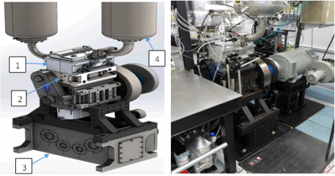
The efficiency of the diesel engine is based on good combustion, and in medium-weight engines, the interactions between the fuel spray and the piston tank walls play a very important role in defining the heat release rate. Staged lip pistons promote turbulence phenomena that are the result of faster and more efficient heat release, but it is important to note that this behavior is more observable for late injection stalls where the engine is not operating at its maximum efficiency [43]. From the above, Figure 1 represents a new medium-weight diesel search engine was carried out at Sandia National Laboratories, to ensure quality research on the combustion of pollutants and methods of heat loss through walls to improve its efficiency. Based on the data from the previous study, our research topic was experimentally validated, Tables 1 and 2 represent respectively the engine parameters and the properties of the injected fuels.
Note: 1-Cast alumium cylinder head; 2-Custom deck adapter facilites conversion to optimal engine; 3-Reconfiguration, belt-driven Lanchester balancing box; 4-Control of intake flow rate, composition, and temper.
Figure 1. Experimental diesel engine [44, 45]
Table 1. Engine parameters
|
Bore×Stoke |
99×109 mm |
|
Displacement engine |
0.477 L |
|
Compression ratio |
16.2 |
|
Nozzle diameter |
0.254 mm |
|
Fuel decane |
C10H22 |
|
Fuel injected per orifice |
29.58 mg/cycle |
|
Injection pressure |
800 bars |
|
Injection start timing |
10 CA |
|
Injection duration |
200 CA |
|
Spray direction |
700 with the cylinder axis |
|
Coordinates of spray emanation point |
x=0, y=0, z=2e-5m |
|
Engine speed |
2000 rpm |
|
Number of nozzles |
7 |
|
Intake valve closed (IVC) |
5700 CA |
|
Exhaust valve opened (EVO) |
8330 CA |
|
Swirl number at IVC |
1.3 |
Table 2. Properties of diesel and methanol fuel [10, 46]
|
Properties |
Diesel |
Methanol |
|
Molecular formular |
C10-C15 |
CH3OH |
|
Molecular weight |
190-220 |
32 |
|
Heat of evaporation [kJ/kg] |
260 |
1178 |
|
Lower heating value [MJ/kg] |
42.5 |
19.7 |
|
Kinematic viscosity at 20℃ [m2/s] |
3.35 |
0.734×10⁻⁶ |
|
Density at 20℃ [kg/m3] |
840 |
790 |
|
Stoichiometric air fuel ratio |
14.7 |
6.45 |
|
Auto ignition temperature [℃] |
316 |
464 |
|
Carbon content [%] |
86 |
37,5 |
|
Hydrogen content [%] |
14 |
12,5 |
|
Oxygen content [%] |
0 |
50 |
|
Sulfur content [%] |
|
- |
|
Flame temperature [℃] |
2054 |
1890 |
|
Flame spread rate |
- |
2-4 |
|
Flame spread rate |
- |
2-4 |
|
Boiling point [℃] |
180-370 |
65 |
|
Research octane Number |
- |
106 |
|
Cetane Number |
51 |
≤5 |
2.2 Methodology
2.2.1 Use of CFD
Computational fluid dynamics (CFD) is a powerful tool for reducing the number of tests required to develop a new process. This is particularly interesting for internal combustion engines, for which bench testing is expensive. In fact, in this domain, where experimental testing is particularly costly and time-consuming, simulations can be a good approach. Although 0D models can be implemented easily, the fact is that they are less efficient than CFD models, which are simply numerical computations applied to fluid mechanics. This consists of solving in a given geometry the fundamental equations of fluid mechanics, which can optionally be coupled to the heat transfer or chemical reaction equations. Indeed, its low cost compared to that of experimental measurements makes it possible to multiply numerical tests. This is usually a first step in the development of a new process for operating automotive engines or the use of new fuels that pose many physical problems requiring modeling. The code and calculation algorithm are shown in Figure 2 below.
Figure 2. Flowchart of the numerical study
2.2.2 Injection profile
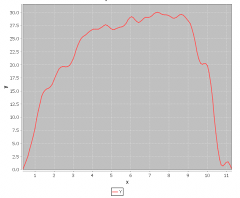
The injection profile presented in Figure 3 is one of the most important parameters in the operation of engines. It provides the injection pressure required for atomization in the combustion chamber and determines the characteristics of combustion. This parameter has a direct impact on fuel consumption, emissions, and engine noise in general. For these effects in simulation work with CFD codes, special care must be paid to the injection profile to ensure a good fit and avoid these phenomena. The injection rate used in this study is that obtained from the Sandia search engine (see Figure 1). We used this data to infer the speed profile. The diagram shown in Figures 4 and 5 represents all the injection characteristics. These characteristics make it possible to give the spray the correct position and orientation in order to stall the problem.
Figure 3. Injection rate profile
Figure 4. Spray tilt angle
Figure 5. 3D view spray location system
2.2.3 Spray orientation
For this study, we not only implemented the standard k-ε turbulence models and the k-ε RNG model in order to understand the phenomenon of turbulence during combustion, but we also calibrated the injection spray from two different angles, allowing us to observe variations in turbulent combustion parameters. The Sandia search engine has been designed to perform laboratory tests with a view to optimizing and promoting the reduction of pollutants from a direct injection diesel engine. The inclination of the jet during design is approximately 61.5° between the cylinder wall and the piston head. For this study, we opted to move the jet closer and farther, about 1.5° around the initial tilt angle. This study was carried out near the initial angle in order to observe variations in the combustion process under the influence of two turbulence models. This allowed us to perform scenarios at 60° and 63°, not far from the initial angle. This is in order to predict better decision-making during the design and positioning of the jet for the optimization or not of combustion. This will allow us to draw conclusions based on the work of Laid and Zoubir [42] or Paryri et al. [47], who present the effect of the inclination of the combustion jet at two angles of inclination around the initial angle of inclination. The results show that by moving the angle of the spray of fuel away from the piston head wall, the wall does not interfere with the path of the spray. This will increase turbulence by creating intense mixing and combustion, hence the influence on pollutants.
2.2.4 Governing equations of CFD
The equations needed to model the flow of the fuel spray and the associated phenomena will be shown in detail.
2.2.5 Eulerian phase
The Eulerian phase contains the vapor phase of the fuel and the ambient air. The behavior of the Eulerian phase is represented by the Navier-Stokes equations: conservation of mass, momentum and energy. For conservation of mass, Eq. (1) is used.
$\frac{\partial \rho_v}{\partial t}+\frac{\partial}{\partial x_i}\left(\rho_{\mathrm{v}} \mathrm{u}_{\mathrm{i}}\right)=\mathrm{S}_{\mathrm{m}}$ (1)
With the density of steam $\rho_{\mathrm{v}}$, The components of Eulerian velocity ui and the term.
Source obtained by droplet evaporation Sm. This term allows the coupling between the Lagrangian and Eulerian phases. The term source makes it possible to add to the Eulerian phase the mass lost during the evaporation of the liquid phase.
For the conservation of momentum, Eq. (2) is used:
$\frac{\partial}{\partial t}\left(\rho_{\mathrm{v}} \mathrm{u}_{\mathrm{i}}\right)+\frac{\partial}{\partial x_i}\left(\rho_{\mathrm{v}} \mathrm{u}_{\mathrm{i}} \mathrm{u}_{\mathrm{j}}\right)=\frac{\partial p}{\partial x_i}+\frac{\partial \tau_{i j}}{\partial x_i}+\mathrm{S}_{\mathrm{t}}$ (2)
With absolute pressure p and the stress tensor $\tau_{i j}$ given by Eq. (3).
$\tau_{i j}=2 \mu S_{i j}-\frac{2}{3} \mu S_{k k} \delta_{i j}=\mu\left(\frac{\partial u_i}{\partial x_j}+\frac{\partial u_j}{\partial x_i}-\frac{2}{3} \frac{\partial u_k}{\partial x_k} \delta_{i j}\right)$ (3)
With the Kronecker symbol $\delta_{i j}$. The term source St comes from the drag force of the droplets and is equal to the inverse of the momentum transfer.
For energy conservation, Eq. (4) is used:
$\begin{aligned} \frac{\partial}{\partial t}\left(\rho_{\mathrm{v}} \mathrm{e}_{\mathrm{t}}\right)+\frac{\partial}{\partial x_j}\left(\rho_{\mathrm{v}} \mathrm{e}_{\mathrm{t}} \mathrm{u}_{\mathrm{j}}\right) & =-\frac{\partial}{\partial x_j}\left(\mathrm{pu}_{\mathrm{j}}\right)+\frac{\partial}{\partial x_j}\left(\tau_{i j} \mathrm{u}_{\mathrm{i}}\right)-\frac{\partial q_i}{\partial x_j}+\mathrm{S}_{\mathrm{e}}\end{aligned}$ (4)
For energy conservation, Eq. (4) is used: et and heat flux $q_i$ are calculated with Eqs. (5) and (6).
$\mathbf{e}_{\mathrm{t}}=\frac{\boldsymbol{p}}{\gamma_v-1}+\frac{1}{2} \mathrm{u}_{\mathrm{i}} \mathrm{u}_{\mathrm{i}}$ (5)
$\boldsymbol{q}_{\boldsymbol{i}}=-\mathrm{k}_{\mathrm{v}} \frac{\partial T}{\partial x_j}$ (6)
With adiabatic index $\gamma_v$ of gas and thermal conductivity index $k_v$ gas. The term heat transfer source $S_e$ is the inverse of heat change caused by evaporation and conduction.
2.2.6 Lagrangian phase
The Lagrangian phase contains the liquid phase of the fuel. This phase is superimposed on the Eulerian phase and transfer terms make it possible to link the two phases. The equation to be solved is that of conservation of momentum.
$\frac{\mathrm{du}_{\mathrm{l}}}{\mathrm{dt}}=\mathrm{F}_{\mathrm{T}}\left(\mathrm{u}_{\mathrm{v}}-\mathrm{u}_l\right)+\mathrm{F}_{\mathrm{MV}}+\frac{g\left(\rho_{\mathrm{l}}-\rho_{\mathrm{v}}\right)}{\rho_{\mathrm{l}}}$ (7)
The momentum contains the forces that are applied to the drop, namely drag force FT, virtual mass FMV and gravity g. The equations for the forces FT and FMV are given by Eqs. (8) and (9).
$\mathrm{F}_{\mathrm{T}}=\frac{18 \mu_{\mathrm{V}}}{\rho_l d_l^2} \frac{C_{\mathrm{D}} R e_{\mathrm{r}}}{24}$ (8)
$\mathrm{F}_{\mathrm{MV}}=\frac{1}{2} \frac{\rho_{\mathrm{r}}}{\rho_{\mathrm{l}}} \frac{\mathrm{d}}{\mathrm{dt}}\left(\mathrm{u}_{\mathrm{v}}-\mathrm{u}_{\mathrm{l}}\right)$ (9)
Relative Reynolds numbers $R e_{\mathrm{r}}$ and drag coefficient CD are calculated with Eqs. (10) and (11).
$\mathbf{C}_{\mathbf{D}, \text { sphère }}=\left\{\begin{aligned} 0.424, & \mathrm{Re}>1000 \\ \frac{24}{R e}\left(1+\frac{1}{6} R e^{2 / 3}\right), & \mathrm{Re} \leq 1000\end{aligned}\right.$ (10)
$R e_{\mathrm{r}}=\frac{\rho_{\mathrm{v}} d_l}{\mu_{\mathrm{v}}}\left(\mathrm{u}_1-\mathrm{u}_{\mathrm{v}}\right)$ (11)
The term drag is the dominant term in the equation, considering the high relative velocity of droplets in ambient air. The virtual mass force is calculated with the inertia of the displaced volume and is proportional to the density of the fluid. Since air is much less dense than fuel, this term is quite weak, and it is possible to overlook it. Since the size of the drops is less than 0.1 mm, the force of gravity is minimal, which also makes it possible to neglect the term gravity. By limiting the equation of the balance of forces to the drag forces, it is possible to write the equation of conservation of momentum as follows:
$\frac{\mathrm{du}_1}{\mathrm{dt}}=\mathrm{F}_{\mathrm{T}}\left(u_y-u_l\right)$ (12)
2.3 Combustion modeling
2.3.1 Standard k-ε model
This model developed by Launder and Spalding [23] is the simplest of the turbulence models generally used in CFDs. The κ-ε model is a semi-empirical model that assumes that the flow is totally turbulent and that the effects of molecular viscosity are negligible. This model uses two transport equations to independently determine turbulent kinetic energy $\kappa$ and its dissipation rate $\varepsilon$ [23]. The model is computationally efficient, robust, and reasonably accurate for many turbulent applications. This model is generally popular in an industrial context. The transport equations of $\kappa$ and $\varepsilon$ are written according to Eqs. (13) and (14).
$\begin{gathered}\frac{\partial \bar{\rho} \tilde{k}}{\partial t}+\nabla \cdot(\bar{\rho} \tilde{u} \tilde{k})=-\frac{2}{3} \bar{\rho} \tilde{u} \nabla \cdot \tilde{u}+(\bar{\sigma}-\Gamma): \nabla \tilde{u}+ \nabla \cdot\left[\frac{\mu+\mu_T}{P r_k} \nabla \tilde{k}\right]-\bar{\rho} \tilde{\varepsilon}+\dot{\bar{W}}^s\end{gathered}$ (13)
$\begin{gathered}\frac{\partial \bar{\rho} \tilde{\varepsilon}}{\partial t}+\nabla \cdot(\bar{\rho} \tilde{u} \tilde{\varepsilon})=-\left(\frac{2}{3} C_{\varepsilon 1}-C_{\varepsilon 3}\right) \bar{\rho} \tilde{\varepsilon} \nabla \cdot \tilde{u} +\nabla \cdot\left[\frac{v+v_T}{P r_{\varepsilon}} \nabla \tilde{\varepsilon}\right]+\frac{\tilde{\varepsilon}}{\tilde{k}}\left[C_{\varepsilon 1}(\bar{\sigma}-\Gamma): \nabla \tilde{u}-C_{\varepsilon 2} \bar{\rho} \tilde{\varepsilon}+C_{\mathrm{s}} \dot{W}^s\right]\end{gathered}$ (14)
In these equations $\operatorname{Pr}_k, \operatorname{Pr}_{\varepsilon}, C_{\varepsilon 1}, C_{\varepsilon 2}, C_{\varepsilon 3}$, are constants of the model. The source terms involved $\dot{\bar{W}}^s$ are calculated based on the droplet probability distribution function. Physically, $\widetilde{\dot{\mathbf{W}}}^{\mathrm{s}}$ is the negative of the rate at which turbulent eddies do a job of dispersing spray droplets. Cs=5 was suggested based on the assumption of retention of the length scale in spray/turbulence interactions.
2.3.2 RNG $\mathrm{k}-\varepsilon$ model
This model is a variation of the standard $\kappa-\varepsilon$ model. The advanced (and recommended) version of the $\mathrm{k}-\varepsilon$ model is derived from group theory (RNG), first proposed by Yakhot et al. [29]. The equation k in the RNG version of the model is the same as in the standard version, but equation ε is based on a rigorous mathematical derivation rather than empirically derived constants. The RNG equation ε is written as follows:
$\begin{gathered}\frac{\partial \bar{\rho} \tilde{\varepsilon}}{\partial t}+\nabla \cdot(\bar{\rho} \tilde{u} \tilde{\varepsilon})=-\left(\frac{2}{3} C_{\varepsilon 1}-C_{\varepsilon 3}\right) \bar{\rho} \tilde{\varepsilon} \nabla \cdot \tilde{u} \\ +\nabla \cdot\left[\frac{v+v_T}{\operatorname{Pr}_{\varepsilon}} \nabla \tilde{\varepsilon}\right]+\frac{\tilde{\varepsilon}}{\tilde{k}}\left[C_{\varepsilon 1}(\bar{\sigma}-\Gamma): \nabla \tilde{u}-C_{\varepsilon 2} \bar{\rho} \tilde{\varepsilon}+\mathrm{C}_{\mathrm{s}} \dot{\bar{W}}^s\right] -\bar{\rho} R c\end{gathered}$ (15)
where, the last term R on the right side of the equation is defined as follows:
$\mathrm{R}=\frac{C_\mu \eta^3\left(1-\frac{\eta}{\eta_0}\right)}{1+\beta \eta^3} \frac{\tilde{\varepsilon}^2}{\widetilde{k}}$ (16)
With
$\eta=\mathrm{S} \frac{\tilde{k}}{\tilde{\varepsilon}}$, (17)
$\mathrm{S}=\sqrt{(2 \bar{S}: \bar{S})}$ (18)
And $\bar{S}$ is the tensor of the mean strain rate,
$\bar{S}=0.5\left(\nabla \tilde{u}+\nabla \tilde{u}^T\right)$ (19)
Compared to the standard ε equation, the RNG model has an additional term, which takes into account non-isotropic turbulence, as described by Yakhot et al. [29].
Model constant values $\operatorname{Pr}_k, \operatorname{Pr}_{\varepsilon}, C_{\varepsilon 1}, C_{\varepsilon 2}, et \, C_{\varepsilon 3}$ used in the RNG version are also shown in Table 3. In the ANSYS Forte implementation, the RNG value of the variable is based on the work of Han and Reitz [31], who modified the constant to account for the compressibility effect.
$C_{\varepsilon 3}=\frac{-1+2 C_{\varepsilon 2}-3 m(n-1)+(-1)^\delta \sqrt{6} C_\mu C_\eta \eta}{3}$ (20)
where, m=0.5, n=1.4 for an ideal gas, and
$\mathrm{R}=\frac{\eta\left(1-\frac{\eta}{\eta_0}\right)}{1+\beta \eta^3}$ (21)
with
$\delta=\left\{\begin{array}{l}1 \text { si } \nabla \tilde{u}<0; \\ 0 \text { si } \nabla \tilde{u}>0.\end{array}\right.$ (22)
Using this approach, the value of $\mathrm{C}_{\varepsilon 3}$ varies in the range of -0.9 to 1.72621, and in ANSYS Forte is determined automatically, depending on the flow conditions and the specification of other constants in the model, η0 et β. Han and Reitz [15] applied their version of the RNG k-ε model to engine simulations and observed improvements in results compared to the Standard Model.
Table 3. Values of constants in turbulence models k-e and RNG-e
|
|
|
$C_{\varepsilon 1}$ |
$C_{\varepsilon 2}$ |
$C_{\varepsilon 3}$ |
|
k-ε standard |
0.09 |
1.44 |
1.92 |
-1.0 |
|
RNG k-ε |
0.0845 |
1.42 |
1.68 |
Eq. 2.19 |
|
|
1⁄Prk |
1⁄Prε |
η0 |
β |
|
k-ε standard |
1.0 |
0.769 |
- |
- |
|
RNG k-ε |
1.39 |
1.39 |
4.38 |
0.012 |
2.3.3 NOx formation model
The mechanism of NO formation has been studied by many researchers.
Zeldovich et al, however, showed the particular role of the following reactions in the formation of NO. The NO concentration is calculated decoupled from the combustion phenomenon, i.e., by a post-treatment procedure, established from the reversible reactions of the Zeldovich mechanism [29]:
$\frac{d[N O]}{d t}=\frac{2 R\left\{1-\left([N O] /[N O]_e\right)^2\right\}}{1+\frac{[N O]}{\left([N O]_e\right) R_1} /\left(R_2+R_3\right)}$ (23)
where, the following notations have been introduced, designating by [ ]e the equilibrium concentrations. The concentration of NO in Eq. (23) can be converted into a mass fraction as:
$\frac{d X_{N O}}{d t}=\frac{2\left(\frac{M_{N O}}{\rho c \cdot v}\right) R_1\left\{1-\left([N O] /[N O]_e\right)^2\right\}}{1+\frac{[N O]}{\left([N O]_e\right) R_1} /\left(R_1+R_3\right)}$ (24)
2.3.4 Soot formation
Concerning soot, an empirical model is used by considering two competing reactions: soot formation and soot oxidation. It is easier to implement with the CFD program because it provides empirical equations that must be adjusted to match the experimental soot profile. One of these most widely used models was proposed in 1983 by Kadota and Hiroyasu [48], directly applicable to engine simulation. This model was implemented by Zhao et al. [49] for developing a diesel engine and is confronted by other models. It follows equations that calculate soot formation rate using soot formation rate and oxidation rate in Arrhenius-type equations:
$\begin{aligned} & \frac{d m_{\text {soot }}}{d t}=\left(\frac{d m_{\text {soot }}}{d t}\right)_{\text {formation }} -\left(\frac{d m_{\text {soot }}}{d t}\right)_{\text {oxydation }}\end{aligned}$ (25)
$\begin{aligned} & \left(\frac{d m_{\text {soot }}}{d t}\right)_{\text {formation }}= \quad A_f m_{\text {fuel }} p^{0.5} \exp \left(-\frac{E_f}{R T}\right)\end{aligned}$ (26)
$\begin{aligned} & \left(\frac{d m_{\text {soot }}}{d t}\right)_{\text {oxydation }}= A_o m_{\text {soot }} X_{o_2} p^{1.8} \exp \left(-\frac{E_o}{R T}\right)\end{aligned}$ (27)
where, $m_{\text {soot }}$ is the mass of net soot formed, $m_{f u e l}$ is the mass of fuel vaporized, $X_O$ is the molar fraction of oxygen, $E_f$ and $E_o$ are the activation energies of soot formation and oxidation, respectively, $A_f$ and $A_o$ are parameters that can be adjusted to match the simulation to the experiment.
2.3.5 The injection model
The KH-RT model suggests that the disturbance of the liquid is due to two types of instabilities: the first instability is of the Kelvin-Helmholtz type Based on the linear theory of instabilities, Reitz obtains the wavelength A_KH and the rate of increase Ω_KH of the fastest growing wave. Based on the dimensionless numbers of the problem, Reitz gets the following correlations [50]:
$A_{K H}=\frac{9.02 r_0(1+0.45 \sqrt{Z})\left(1+0.4 T_a^{0.7}\right)}{\left(1+0.865 W e^{1.67}\right)^{0.7}}$ (28)
$\Omega_{K H}=\frac{0.34+0.38 W e^{1.5}}{(1+Z)\left(1+1.4 T^{0.6}\right)} \sqrt{\frac{\sigma}{\rho_l r^3}}$ (29)
2.3.6 Initial and boundary conditions
The initial and boundary conditions make it possible to specify the size or scope of the models when solving problems. They also describe the phenomena of these models, then detail the new phenomena and link models from different theoretical contexts of physics. In order to carry out simulations of this study, it is necessary to apply the initial conditions and the limits below in Table 4.
Table 4. Initial and boundary conditions
|
Variable |
Value |
|
Initial gas temperature |
372.12 K |
|
Pressure |
1.5 bar |
|
Initial swirl ratio |
1.5 |
|
Initial swirl profile factor |
3.11 |
|
Turbulence Kinetic energy |
10000 cm2/sec |
|
Piston temperature |
500 K |
|
Sector angle |
51.42 deg |
|
Head temperature |
470 K |
|
Liner temperature |
420 K |
|
Water injection pressure |
40 bars |
3.1 Model validation
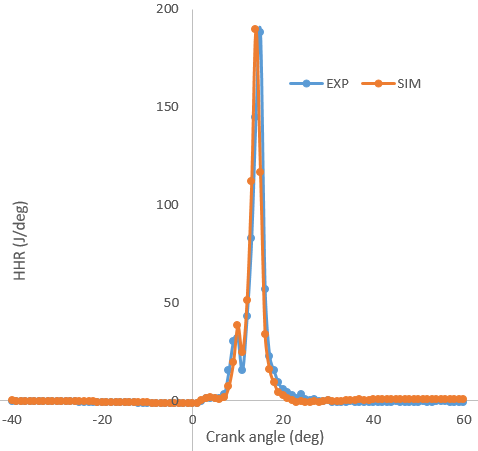
The simulated model of this engine has been validated using the previously mentioned experimental data from the literature. This engine is operating at 2000 rpm; an IMEP of 1 MPa was chosen for this numerical study. Figures 6 and 7 below show the validation of the measured and calculated cylinder pressure and heat release curves. We can see that the correspondence of the heat release curve is good for validation. Although it presents higher estimates of heat release as compared to the initial heat release, this model predicts the trend of cylinder pressure and heat release rate, as well as the overall characteristics of combustion. The expected ignition delay period, the combustion time and all parameters of the diesel engine are contained in the Table 1.
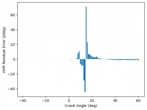
The least squares method allowed us to present the distribution of cylinder pressure validation error and heat release rate. It can be observed for these two cases that this error is relatively greater between 10 to 20 degrees crankshaft angle (Figure 8). It is estimated at about 11% for the cylinder pressure over the entire distribution and about 9% for the rate of heat release (Figure 9). The work of Ngayihi Abbe et al. [51] on the simulation of Neem combustion in a diesel engine, to predict pollutants, validates the cylinder pressure, temperature and pollutants, then reveals that during the validation process between the numerical simulation and experimental study, the error interval after calculation should not be greater than 15%.
Figure 6. Validation of cylinder pressure
Figure 7. Validation of heat release rate
Figure 8. Residual error for pressure
Figure 9. Residual error for heat release rate
3.2 Results analysis
Overall, there is a variation in combustion parameters (cylinder pressure, heat release, and temperature) and pollutant emissions. Particular attention is paid to the fact that in the representations below, some results give the impression of being missing, although they are confused with others. This is due to the fact that their representation is made at a wider portion around the angle of the crankshaft. In addition, the choice of moving closer and further away from the spray by 1.5° around the initial injection and then the application of the two turbulence models can contribute to a tendency to superimpose the results. In order to better visualize, a portion of these results has been included in the appendix of this work.
Figure 10. Cylinder pressure variation
Figure 11. Heat release rate variation
To understand the effect of the turbulence model and consequently the variation of the pressure cylinder, the rate of heat release, and pollutant emissions, an injection of methanol (CH3OH) is made at 25% and 50% of the two models of turbulence: k-ε RNG and standard k-ε at two spray tilt angles of 60° and 63°. Figures 10 and 11 show the variations in cylinder pressure and heat generation for the injection of the single diesel and then the simultaneous injection of the diesel and methanol. For diesel injected alone at 60° and 63° of spray inclination, a high peak can be observed for the inclination of 60. This is because the closer the spray is to the piston head, the less turbulence there is. This is in line with the work of Laid and Zoubir [42], who concludes that the variation of the angle of the spray, even at a small angle, causes the combustion parameters to vary. This result also shows an increase in cylinder pressure and heat release rate of approximately 10% and 25%, respectively, for the M+D mixture at 2000 rpm to 25% and 50% for any spray tilt angle and for any turbulence model used. The variation in the peak could be explained by the fact that an appropriate advanced timing of diesel injection results from the cooling effect of the injected methanol [10]. The pressure in the cylinder increases with the percentage of methanol injection due to the timing of the absorption of the advanced timing of diesel injection, which results from the absorption of greater compressive heat by the presence of excess methanol [10].
The pressure in the cylinder increases with the percentage of methanol injection due to the start-up moment of the absorption of the advanced timing of the diesel injection, which results from the absorption of more heat of compression by the presence of excess methanol [10]. During this period, the advanced timing of diesel injection with the increase in the percentage of methanol injection also allows enough time for diesel fuel to mix with the methanol and air, resulting in a less homogeneous charge and allowing less fuel to burn during the premixed combustion phase. This also explains the decrease or increase in the rate of heat release with an increase in the percentage of methanol injection [10].
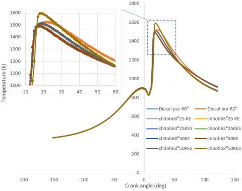
3.3 Temperature variation
Figure 12 illustrates the evolution of the average temperatures of a conventional diesel and diesel methanol mixture inside the cylinder during a cycle. The injection begins at 10° of the crankshaft angle after the top dead center, and according to the previous curves, combustion begins after TDC with an auto ignition time of about 11° crank angle. The rapid combustion of air and fuel mixtures during the delay period causes a sudden rise in pressure, temperature, and heat release rate. During the induction stroke, temperature remains constant, then slightly increases by 15% during the compression stroke, and just before TDC at the compression phase, there is a small drop in temperature due to the influence of diesel injected cold into the combustion chamber. Then the temperature drops during the power and exhaust strokes to its initial value. The maximum average temperature reached is more than 1500 K, which is that of the injection of methanol at 50% for the RNG k-ε model. This means that the increase in temperature and even some pollutants are a function of the increase in the methanol injection rate, which, in accordance with the work of Therefore, when adding methanol to the diesel engine, the cuts must be executed judiciously in order to better control the combustion and consequently the temperature. Note that the injector nozzle used in this k-ε RNG model has 60° and 63° inclination spray angles slightly above those of the standard k-ε model [38]. This shows that increasing the inclination spray angle consequently leads to an increase in temperature by moving the spray of fuel away from the wall of the cylinder as it does not manage the spray pattern. Li et al. [52] and Nang Nkol et al. [53] state in their study that the geometry of the piston bowl brings total changes in the combustion phenomenon resulting from the large vortex. This may therefore explain the discrepancies between the different injections of methanol.
It is important to note that the fuel injected is dispersed differently in the combustion chamber due to the two injectors simultaneously injecting diesel and methanol at different spray angle positions. The differences in cylinder pressure, heat release, temperature, and possibly pollutants are also due to the differences in turbulence models applied. This can be explained by the fact that the spray generates turbulence, and the intensity of this turbulence begins to increase at the top dead center for both turbulence models. The variation in the parameters observed in this study is therefore understandable because it is stated in the literature that the spray does not significantly change the length scale, which justifies the terms of the spray equation [31]. Comparing the two cases, it can be said that these differences are more visible after 10 degrees before TDC, probably because the turbulence intensity and the turbulence scale for Cε3=-1.0 are smaller than those obtained in Eq. (20). These differences in turbulence characteristics significantly influence the prediction of combustion parameters and pollutant emissions, hence the differences observed on curves.
Figure 12. Temperature variation for different models with spray angle tilt
3.4 Evolution of pollutants
3.4.1 Carbon monoxide
Figures 13, 14, and 15 show the carbon monoxide content of diesel alone and the diesel methanol blend for two models of turbulence and at crankshaft angles of 60° and 63° of the spray. It can be noted that the peak of carbon monoxide is higher by about 10% to 60% for the D+M mixture during the injection phase, but during the diffusion phase, we can notice a considerable decrease in carbon monoxide of about 60% between diesel and the injected D+M mixtures. According to Chao et al. [13], their work showed an increase in the level of CO, and this increase was estimated at about 126% at low engine speed and 43% at high load (high engine speed). On the other hand, Huang et al. [54] describe the opposite in their study and note a decrease in CO emissions. It is very important to say that CO is the result of improper mixtures and incomplete combustion, as it is controlled primarily by the air/fuel ratio [10]. According to Figure 11, the temperature of the gas in the D+M engine may be lower or higher depending on the ratio of the D+M mixture injected into the conventional diesel engine, which may be explained by the fact that as the temperature of the flame decreases, a quenching layer may be created and a greater amount of methanol may be within the range of the rich air/fuel ratio or even in the liquid state in the extinguishing layer because the flame front spreads quite slowly [10]. Increasing the ignition time is also a reason to increase CO emissions, which is explained by the fact that it causes fuel combustion in the expansion stroke, which lowers the temperature of the gases and reduces the CO oxidation reaction time, leading to incomplete combustion and relatively higher CO emissions [10]. This is consistent with the work of [10], but is opposed to the results of Lyon et al. [55]. This opposition can be explained by the combustion time, which is not proportional, and the flow rate of the injected methanol. The influence of the tilt angle of spray and turbulence models can be noticed, which also play an important role in controlling CO emissions. For a fixed angle of 60°. There is an increase in carbon monoxide in the standard k-ε model compared to the k-ε RNG model; on the other hand, there is a decrease in monoxide. By comparing these pollutants at two different angles and two different models, as shown in the figures below, a significant variation is observed. This variation is about 10% to 60% during the combustion phase after injection and at 10 degrees after TDC. This variation favors in a number of cases the RNG k-ε turbulence model compared to the standard model, although the opposite is produced in other cases and would be explained by other parameters later.
Figure 13. Carbon monoxide
Figure 14. Carbon monoxide has 60° spray tilt
Figure 15. Carbon monoxide at 63° spray tilt
3.4.2 Nitric oxide
The monoxide formation of nitric oxide is governed primarily by the maximum cylinder temperature and the crankshaft angle at which it occurs. Figures 16, 17, and 18 below show the comparison of the nitric oxide of the conventional diesel engine on the one hand and the engine with injection of the D+M mixture on the other hand. The standard k-ε and k-ε RNG turbulence models and the angles 60° and 63° are used and then compared with each other. There is an increase in NO in conventional diesel compared to that of the D+M mixture during the premix combustion phase. This difference is visible in the figures below and is estimated at 30% of the peak value of diesel and at the minimum value of the D+M mixture. Although this decrease in NO is more observable in Figures 16 and 17, it can also be seen that at 50% methanol injection, the decrease in NO is greater, which shows the impact of the spray tilt angle on the evolution of this pollutant. The reduction of NO in the mixture can be explained by the lower cylinder temperatures produced due to the cooling effect of the mixture. Anand et al. [56] obtained from their work a reduction in NO of about 37.3% under full load and concluded that smoke formation occurs in the diffusion combustion phase and is governed by the air/fuel ratio, the spraying properties of the fuel, and the combustion temperature.
Figure 16. Nitric oxide
Figure 17. Nitric oxide at 60° spray tilt
3.4.3 Nitrogen dioxide
Figures 19, 20 and 21 show the variation of NO2 to different percentages of methanol 25% and 50% implemented. The NO2 concentration is obtained by removing the NO concentration from the NOx concentration [57]. We can notice a significant increase in the concentration of NO2 in the exhaust gases when using the D+M mixture as it increases approximately to 20% between the maximum of the D+M mixture and that of pure diesel fuel. The increase in NO2 is quite significant when comparing the pure diesel and the case of methanol at 50% compared to 25%. In this case, it can be said that the increase in methanol immediately leads to an increase in the concentration of NO2, but the percentage increased, is less significant which indicates a decrease in the influence rate. It has been shown that the oxidation of methanol in NO can lead to the formation of NO2 emissions, methanol functioning as a source of HO2 free radicals [55, 57, 58]. The same reason may have led to the increase in NO2 emissions in our study Hence a converging conclusion with the work of the latter. It is important to note that with methanol, the engine load has a direct impact on the increase or decrease in NO2 as it has been seen that there is poor combustion of methanol at low loads compared to the improved combustion of methanol at higher loads. It is then possible to say unburnt hydrocarbons contain more methanol at low loads than at higher loads and that NOx increases with increase in engine load. Knowing that NO2 has an adverse impact on human health at high concentrations and over time, it is therefore important to say that the increase in NO2 emissions associated with methanol should be a call for concern.
Figure 18. Nitric oxide has 63° spray tilt
Figure 19. Nitrogen dioxide
Figure 20. Nitrogen dioxide 60° spray tilt
Figure 21. Nitrogen dioxide has 63° spray tilt
3.4.4 Nox and soot
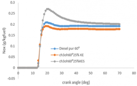
The change in NOx emissions is shown in Figures 22, 23, and 24. The simulations are carried out at 2000 rpm and with two different percentages of methanol injected at 25% and 50%. The reduction is about 10% to 60% for adding methanol, then an increase in the diesel injection is inclined to 600. It is generally observed that increasing the engine load automatically increases NOx emissions with the engine running on pure diesel or D+M [57]. When compared to the conventional engine, NOx emissions with the D+M mixture are reduced. For this study, the increase in the methanol addition rate thus leads to a decrease in NOx, which corresponds to the work of Soni and Gupta [59], which makes cuts of 5% to 30% of methanol compared to diesel. Several factors can lead to NOx emissions, for example, when methanol is ignited when diesel fuel is injected. Firstly, an increase in oxygen supply could increase NOx emissions. In addition, due to its high latent heat of evaporation, methanol tends to absorb more heat than diesel fuel and thus lowers the combustion temperature, resulting in reduced NOx emissions [57]. Studies show that methanol can lead to an increase in ignition time, resulting in an increase in fuel consumption during the premixed phase [54] and thus an increase in combustion temperature. These positive and negative phenomena compete with each other and could lead to an increase or decrease in NOx emissions. Huang et al. [54] demonstrate that there was both an increase and a decrease in NOx emissions under different operating conditions. Chao et al. [13] performed two steady-state tests, one at high engine load and the other at low engine load, using up to 15% volume of methanol. Their work showed that the maximum reduction in NOx emissions was 9% at high engine loads and 26% at low engine loads. The reduction value is similar to that obtained in our study. It is obvious that at high load, the temperature of the gas inside the cylinder is higher during the intake process, which will weaken the effect of methanol on lowering the combustion temperature. Moreover, at high loads, the excess air ratio will be much lower, and thus the oxygen in methanol molecules will play a more important role in the formation of NOx. Thus, compared to low engine load and medium load conditions, we can say that the NOx reduction effect is weakened.
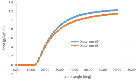
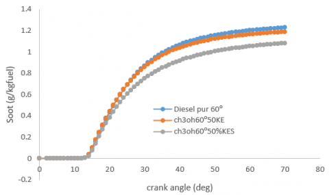
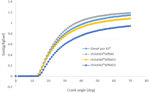
As for Figures 25, 26, and 27, they show the variation of soot. We can notice a dominance of conventional diesel over the D+M mixture on the one hand, and on the other hand, the opposite occurs in some cases. Figures 22 and 23 show that the injection of pure diesel fuel at an inclination spray angle of 60° increases soot. A difference is estimated at 40% between this diesel injection and the minimum injection of D+M mixtures. On the other hand, Figure 24 shows the opposite, as we can observe an increase in soot in the D+M mixture of about 22% this is in phase and then in contradiction with the work of Jin et al. [60]. This contradiction can be explained by the difference in the turbulence models applied, the methanol injection rate, to the regime whose scenarios are executed and depending on the angle of inclination of the spray. From Figures 22 and 23, at a fixed angle of 63°, there is an increase in soot at the engine exhaust and a decrease in Nox, which shows a favorable reduction with the RNG k-ε model after injection, that’s to say 10 degrees after BTDC. With injection, the synchronization delay is predicted in both cases. However, the magnitude of the predicted soot is affected by the compressibility flow in the turbulence model. For this same angle of inclination of spray, and in comparison, with the two models of turbulence (Figures 20 and 21), it appears that the NOx decreases by 5%-11% and the soot from the RNG k-ε turbulence model increases by 5%-10% compared to the standard k-ε model. However, the opposite happens for fixed tilt angles and/or fixed models. This can be seen on Soot at 60°.
Figure 22. NOx
Figure 23. NOx has 60° spray tilt
At the end of Figures 20, 21, 22, and 23, it is found that varying the angle of inclination for any turbulence model results in a significant variation of nox and soot, which occurs by reducing the nox in a greater number of cases and increasing the soot. The opposite case is produced in other scenarios; this can be explained by the fact that the shape of the piston bowl plays an important role in the distribution of pollutants. Moreover, increasing the angle of inclination of the spray according to the work of Tian and Wong [61] increases the temperature inside the cylinder, which leads to an increase in the amount of nitric oxide produced. The variation of results obtained explains that taking into account the details of a turbulence model, given their complexity, the spray inclination angle is necessary during the development of models to predict the pollutant emissions of diesel engines. As noted above, the differences observed in Figures 22 and 23 are due to the effect of flow expansion terms in the turbulence model.
Figure 24. NOx has 63° spray inclination
Figure 25. Soot
Figure 26. Soot at 60° spray inclination
3.4.5 Unburned hydrocarbons
Figures 28, 29, and 30 show the evolution of unburnt hydrocarbons during the combustion phase. It is seen that there is not much difference between the D+M mixture and the conventional pure diesel, but a slight increase of about 5–10% of unburnt hydrocarbons in the D+M compared to the conventional diesel. Several studies have shown an approximately 90% increase in HC emissions under low and high load conditions [10, 13]. On the other hand, the work of Huang et al. [54] and Yilmaz [62] described that there was no significant difference in HC emissions from the combustion of methanol and diesel, although the percentage of methanol injected remains an important factor to be considered. It can therefore be concluded that the work of Huang et al. [54] is in line with this study for almost a concordance of the hydrocarbons, which do not change significantly, but is opposed to the work of Chen et al. [57], whose increase is about 90%. This can be due to several parameters, such as the quantity of methanol injected, the range of speed injected, and the quality of the combustion obtained. Fumigation or the addition of methanol may result in increased HC emissions compared to the premixed approach with diesel and methanol [10]. When combustion is incomplete, this can lead to an increase in the level of unburnt hydrocarbon emissions [62]. Yao et al. [10, 63] at the end of their research claim that the lower temperature of the D+M mixture makes combustion incomplete, especially when the level of injected methanol is low, which could result in a lean air + methanol mixture burning at low engine loads. In addition, several locations within the engine, including the clearance volume, are responsible for retaining a quantity of D+M mixture that could not be burned until it escapes from these locations in the exhaust process and contribute significantly to the increased rate of emission of unburnt hydrocarbons [10, 63].
Figure 27. Soot at 63° spray tilt
Figure 28. Unburned hydrocarbons
Figure 29. Unburned hydrocarbons at 60° spray tilt
Figure 30. Unburned hydrocarbons at 63° inclination of the spray
Computational fluid dynamics can be used to predict combustion parameters and pollutant emissions in the case of the internal combustion engine. It is therefore linked in parallel with the experimental and the digital for validation reasons, which gives relevance to the latter because its rendering tends towards the real and the concrete. For this study, a CFD simulation was performed to analyze the injection effect of methanol and the angle of inclination of the spray based on the implementation of the standard k-ε and k-ε RNG turbulence models to predict the combustion parameters and pollutant emissions of a diesel engine running at 2000 RPM. A CFD model was made and validated with the experiment, and then comparisons were made between the combustion parameters resulting from the calculation and the pollutant emissions. The results show the significance that exists when adding methanol to diesel and varying the spray inclination angle in a diesel engine. The results also show that when methanol is injected into a compression-ignition engine, its injection rate greatly influences combustion by acting on temperature and consequently on pollutant emissions. It appears that the choice of turbulence model to adapt for modeling and the spray inclination angle are steps of rigor because of their choice in order to decide the quality of the prediction of combustion parameters and pollutants. In the case of this study, it follows that the RNG k-ε model reduces NOx and other pollutants at the exhaust of an internal engine, although soot showed the opposite with a slight increase. It has been seen that the geometry of the piston bowl and the spray angle play a great role in the combustion parameters. Turbulence in an internal combustion engine can be a difficult task to control, so taking into account its behavior would be wise for future studies. For better analysis, the inclination angles of the spray can be chosen over several steps by moving them closer and further away from the initial angle.
This work was funded by the University of Douala and the Ministry of Higher Education of Cameroon.
|
CFD |
Computational fluid dynamics |
|
BTDC |
After top dead center |
|
ATDC |
Before top dead center |
|
RNG |
Re-Normalization Group |
|
CH3OH |
Methanol |
|
D+M |
Diesel/Methanol |
|
NO2 |
Nitrogen dioxide (g/kgfuel) |
|
NO |
Nitric oxide (g/kgfuel) |
|
CO |
Carbon monoxide (g/kgfuel) |
|
NOx |
Nitrogen oxyde (g/kgfuel) |
|
HC |
Hydrocarbons |
[1] Som, S., Aggarwal, S.K. (2010). Effects of primary breakup modeling on spray and combustion characteristics of compression ignition engines. Combustion and Flame 157(6): 1179 https://doi.org/10.1016/j.combustflame.2010.02.018
[2] Bardi, M., Bruneaux, G., Malbec, L.M. (2016). Study of ECN injectors’ behavior repeatability with focus on aging effect and soot fluctuations. SAE Technical Paper, 2016-01-0845. https://doi.org/10.4271/2016-01-0845
[3] Payri, R., Salvador, F.J., Gimeno, J., Peraza, J.E. (2016). Experimental study of the injection conditions influence over n-dodecane and diesel sprays with two ECN single-hole nozzles. Part II: Reactive atmosphere. Energy Conversion and Management, 126: 1157-1167. https://doi.org/10.1016/j.enconman.2016.07.079
[4] Panao, M., Moreira, A.L.N. (2015). A systematic approach to model and interpret secondary atomization emerging ˜from spray-wall impact in IC Engines. In SPEIC14 - Towards Sustainable Combustion, Lisbon, Portugal.
[5] Fansler, T.D., Trujillo, M.F., Curtis, E.W. (2020). Spray-wall interactions in direct-injection engines: An introductory overview. International Journal of Engine Research, 21(2): 241-247. https://doi.org/10.1177/1468087419897994
[6] Picke, L.M., Lopez, J.J. (2005). Jet-wall interaction effects on diesel combustion and soot formation. Technical Paper, 2005-01-0921. https://doi.org/10.4271/2005-01-0921
[7] NGAYIHI ABBE Claude Valery. Contribution à la modélisation 0D de la combustion Diesel: Application au Biodiesel. Laboratoire Engineering Civil Et Mecanique, (2015-2016). https://www.researchgate.net/profile/Ngayihi-Claude-Valery/publication/311067007_Contribution_a_la_modelisation_0D_de_la_combustion_Diesel_Application_au_Biodiesel/links/5b68444d92851ca497cd21ac/Contribution-a-la-modelisation-0D-de-la-combustion-Diesel-Application-au-Biodiesel.pdf, accessed on June 22, 2023.
[8] Wang, Y., Dong, P.B., Long, W.G., Tian, J.P., Wang, Q.M., Cui, Z.C., Li, B. (2022). Characteristic of evaporation spray for direct injection methanol engine: Comparison between methanol and diesel spray. Processes, 10(6): 1132. https://doi.org/10.3390/pr10061132
[9] Gong, Y.F., Liu, S.H., Li, Y. (2007). Investigation on methanol spray characteristics. Energy Fuel, 21(5): 2991-2997. https://doi.org/10.1021/ef0605089
[10] Yao, C.D., Cheung, C.S., Cheng, C.H., Wang, Y.S., Chan, T., Lee, S. (2007). Effect of Diesel/methanol compound combustion on Diesel engine combustion and emissions. Energy Conversion and Management, 49(6): 1696-1704. https://doi.org/10.1016/j.enconman.2007.11.007
[11] Song, R.Z., Liu, J., Wang, L., Liu, S.H. (2008). Performance and emissions of a diesel engine fueled with methanol. Energy Fuels, 22(6): 3883-3888. https://doi.org/10.1021/ef800492r
[12] Wang, Q.G., Wei, L.J., Wang, P., Yao, C.D. (2015). Investigation of operating range in a methanol fumigated diesel engine. Fuel, 140: 164-147. https://doi.org/10.1016/j.fuel.2014.09.067
[13] Chao, M.R., Lin, T.C., Chao, H.R., Chang, F.H., Chen, C.B. (2001). Effect of methanol-containing additive on emission characteristics from a heavy-duty diesel engine. Science of the Total Environment, 279(1-3): 167-179. https://doi.org/10.1016/S0048-9697(01)00764-1
[14] Jia, Z., Denbratt, I. (2018). Experimental investigation into the combustion characteristics of a methanol/diesel heavy duty engine operated in RCCI mode. Fuel, 226: 745-753. https://doi.org/10.1016/j.fuel.2018.03.088
[15] Han, Z., Reitz, D. (2012). Turbulence modeling of inernal combustion engines using RNG κ-ε models. Combustion Science and Technology, 106(4-6): 267-295. https://doi.org/10.4271/2012-01-0140
[16] Amsden, A.A., O'Rourke, P.J., Butler, T.D. (1989). KIVA-II: A computer program for chemically reactive flows with sprays. Los Alamos National Lab. (LANL), Los Alamos, NM, United States.
[17] Kong, S., Reitz, D. (1993). Multidimensional modeling of diesel ignition and combustion using a multistep kinetics model. Journal of Engineering for Gas Turbines and Power, 115(4): 781-789. https://doi.org/10.1115/1.2906775
[18] Bourgeois, J.A., Martunuzzi, R.J., Savory, E., Zhang, C., Roberts, D.A. (2010). Assessment of turbulence model prediction for an Aero-engine centrifugal compressor. Journal of Turbomachinery, 133(1): 011025. https://doi.org/10.1115/1.4001136
[19] Buhl, S., Diestzsch, F., Buhl, C., Hasse, C. (2017). Comparative study of turbulence models for scale-resolving simulation of internal combustion engine flows. Computers & Fluids, 156: 66-80. https://doi.org/10.1016/j.compfluid.2017.06.023
[20] Reitz, R.D., Rutland, C.J. (1995). Development and testing of diesel engine CFD models. Progress in Energy and Combustion Science, 21(2): 173-196. https://doi.org/10.1016/0360-1285(95)00003-Z
[21] Wang, B.L., Miles, P.C., Reitz, R.D., Han, Z.Y., Patersen, B. (2011). Assessment of RNG turbulence modeling and the development of a generalized RNG closure model. Technical Paper, 2011-01-0829. https://doi.org/10.4271/2011-01-0829
[22] El Tahry, S., Haworth, D. (1992). Directions in turbulence modeling for In-cylinder flows in reciprocating engines. In 29th Aerospace Sciences Meeting, Reno, NV, U.S.A. https://doi.org/10.2514/6.1991-516
[23] Launder. B., Spalding, D.B. (1972). Mathematical Models of Turbulence. Academic Press Inc.
[24] Gosman, A.D., Watkins, A.P. (1977). A computer prediction method for turbulent flow and heat transfer in piston-cylinder assemblies. In Proceedings of the Symposium on Turbulent Shear Flows, Vol. I, Pennsylvania State University, University Park, PA, United States.
[25] Reynolds, W. (1980). Modeling of fluid motion in engines- A introductory overview. https://www.semanticscholar.org/paper/Modeling-of-Fluid-Motions-in-Engines%E2%80%94An-Overview-Reynolds/09653cb6527f2d1e4f120c199e44d6fff39ea99b.
[26] Morel, T., Mansour, N.N. (1982). Modeling of turbulence in internal combustion engine. Technical Paper, 820040. https://doi.org/10.4271/820040
[27] Ramos, J.I., Sirignano, W.A. (1980). Axisymmetric flow model with and without swirl in a piston-cylinder arrangement with idealized valve operation. Technical Paper, 800284. https://doi.org/10.4271/800284
[28] Grasso, F., Bracco, F.V. (1983). Computer and measured turbulence in axisymmetric reciprocating engine. AIAA Journal, 21(4). https://doi.org/10.2514/3.8119
[29] Yakhot, V., Orszag, S.A., Thangam, S., Gatski, T.B., Speziale, C.G. (1986). Development of turbulence models for shear flows by a double expansion technique. Physics of Fluids, 4(7): 1510-1520. https://doi.org/10.1063/1.858424
[30] Choudhury, D., Kim, S.E., Flannery, W.S. (1993). Calculation or turbulence separated flows using a renormalization group besel k-ε turbulence model. Sep. Flows ASME FED, 149: 177-187. https://doi.org/10.1299/kikaib.64.2868
[31] Han, Z., Reitz, R.D. (1995). A RNG k-ε model with appilcation to diesel combustion modeling. Combustion Science and Technology, 106(4-6): 267-295. https://doi.org/10.1080/00102209508907782
[32] Broatch, A., Novella, R., Gracia-Tíscar, J., Gomez-Soriano, J., Pal, P. (2022). Investigation of the effects of turbulence modelind on the prediction of compression-ignition combustion unsteadiness. Sage Journals, 23(4). https://doi.org/10.1177/1468087421990478
[33] Yang, Q.R. (2021). A quasi-dimensional charge motion and turbulence model for combustion and emissions prediction in diesel engines with a fully variable valve train. A Quasi-dimensional Charge Motion and Turbulence Model for Combustion and Emissions Prediction in Diesel Engines with a fully Variable Valve Train, Wissenschaftliche Reihe Fahrzeugtechnik Universität Stuttgart, Springer Vieweg, Wiesbaden. https://doi.org/10.1007/978-3-658-35774-0_3
[34] Barbato, A., Fontanesi, S., D'AdamoWorks by Alessandro D'Adamo, A. (2021). Impact of grid density and turbulence model on the simulation of in-cylinder turbulent flow structures-application to the Darmstadt engine. Technical Paper, 2021-01-0415. https://doi.org/10.4271/2021-01-0415
[35] Ma, J., Liu, HS., Liu, L., Xie, M.Z. (2021). Simulation study on the cryogenic liquid nitrogen jets: Effects of equations of state and turbulence models. Cryogenics, 117: 103330. https://doi.org/10.1016/j.cryogenics.2021.103330
[36] Zhou, L., Zhao, W.H., Luo, H.K., Jia, M., Wei, H.Q., Xie. M.Z. (2021). Spray-turbulence-chemistry interactions under engine-like conditions. Progress in Energy and Combustion Science, 86: 100939. https://doi.org/10.1016/j.pecs.2021.100939
[37] Fang, T.G., Coverdill, R.E., Lee, C.F., White, R.A. (2008). Effects of injection angles on combustion processus using multiple injection strategies in an HSDI diesel engine. Fuel, 87(15-16): 3232-3239. https://doi.org/10.1016/j.fuel.2008.05.012
[38] Kim, H.J., Park, S.H., Lee, C.S. (2016). Impact of fuel spray angles and injection timing on the combustion and emission characteristics of a high-speed diesel engine. Energy, 107: 572-579. https://doi.org/10.1016/j.energy.2016.04.035
[39] Payri, F., Payri, R., Bardi, M., Carreres, M. (2014). Engine combustion network; Influence of de the gas properties on the spray penetration and spreading angle. Experimental Thermal and Fluid Science, 53: 236-243. https://doi.org/10.1016/j.expthermflusci.2013.12.014
[40] Shu, J., Fu, J.Q., Liu, J.P., Ma, Y.J., Wang, S.Q., Deng, B.L., Zeng, D.J. (2019). Effect of injector spray angle on combustion and emissions characteristics of a naturel gas-diesel dual fuel engine based on CFD coupled with reduced chemical kinetic model. Applied Energy, 233-234: 182-195. https://doi.org/10.1016/j.apenergy.2018.10.040
[41] Yoon, S.H., Cha, J.P., Lee, C.S. (2010). An investigation of the effects of spray angle and injection strategy on dimethyl ether (DME) combustion and exhaust emission characteristics in a common-rail diesel engine. Fuel Processing Technology, 91(11): 1364-1372. https://doi.org/10.1016/j.fuproc.2010.04.017
[42] Laid, M., Zoubir, N. (2015). Effet de langle dinclinaison de linjecteur sur la combustion et les emissions des polluants dans un moteur diesel. In 16èmes Journées Internationales de Thermique (JITH 2013), Marrakech, Morocco.
[43] Pastor, J.V., García, A., Micó, C., Lewiski, F., Vassallo, A., Pesce, F.C. (2021). Effect of a novel piston geometry on the combustion process of a light-duty compression ignition engine: an optical analysis. Energy, 221: 119764. https://doi.org/10.1016/j.energy.2021.119764
[44] Nang Nkol, F.P., Issondj Banta, N.J., Offole, F., Ngayihi Abbe, C.V., Mouangue, R. (2022). Effect of direct water injection on emission of pollutants in a diesel engine using CFD and water/fuel mass ratio based parametric analysis. Research Article. https://doi.org/10.21203/rs.3.rs-2214173/v1
[45] Stephen, B. (2020). Sandia's new medium-duty diesel research engine: And what we’re going to do with it. In Conference: Proposed for presentation at the AEC MOU Program Review Meeting, Livermore, CA, USA.
[46] Chen, C.H., Cheung, C.S., Chan, T.L., Lee, S.C., Yao, C.D. (2007). Experimental investigation on the performance, gaseous and particulate emissions of a methanol fumigated diesel engine. Science of The Total Environment, 389(1): 115-124. https://doi.org/10.1016/j.scitotenv.2007.08.041
[47] Payri, R., Bracho, G., Martí-Aldaraví, P., Viera, A. (2017). Near field visualization of diesel spray for different nozzle inclination angle in non-vaporizing conditions. Atomization and Sprays, 27(3): 251-267. https://doi.org/10.1615/AtomizSpr.2017017949
[48] Kadota, T., Hiroyasu, H. (1984). Soot concentration measurement in a fuel droplet flame via laser light scattering. Combustion and Flame, 55(2): 195-201. https://doi.org/10.1016/0010-2180(84)90027-0
[49] Zhao, F.Y., Yang, W.M., Yu, W.B. (2020). A progress review of practical soot modelling development in diesel engine combustion. Journal of Traffic and Transportation Engineering, 7(3): 269-281. https://doi.org/10.1016/j.jtte.2020.04.002
[50] Han, Z., Reitz, R.D. (1994). Turbulence modeling of internal combustion engines using RNG κ-ε models. Combustion Science and Technology, 106(4-6): 267-295. https://doi.org/10.1080/00102209508907782
[51] Ngayihi Abbe, C.V., Nzengwa, R., Danwe, R., Ayissi, Z.M., Obonou, M. (2015). A study on the 0D phenomenological model for diesel engine simulation: Application to combustion of Neem methyl esther biodiesel. Energy Conversion and Management, 89: 568‑576. https://doi.org/10.1016/j.enconman.2014.10.005
[52] Li, J., Yang, W.M., An, H., Maghbouli, A., Chou, S.K. (2014). Effects of piston bowl geometry on combustion and emission characteristics of biodiesel fueled diesel engines. Fuel, 120: 66-73. https://doi.org/10.1016/j.fuel.2013.12.005
[53] Nang Nkol, F.P., Issondj Banta, N.J., Ngayihi Abbe, C.V., Mouangue, R. (2023). CFD Study of the effect of engine speed on the combustion process and the formation of pollutants in a diesel engine. International Journal of Engineering Trends and Technology, 71(10): 163-172. https://doi.org/10.14445/22315381/IJETT-V71I10P215
[54] Huang, Z.H., Lu, B.H., Jiang, D.M., Zeng, K., Liu, B., Zhang, J.Q. (2004). Engine performance and emissions of a compression-ignition engine operating on the diesel/methanol blends. Proceedings of the Institution of Mechanical Engineers, Part D: Journal of Automobile Engineering, 218(4): 1011-1024. https://doi.org/10.1243/095440704773599944
[55] Lyon, R.K., Cole, J.A., Kramlich, J.C., Chen, S.L. (1990). The selective reduction of SO3 to SO2 and oxidation of NO to NO2 by methanol. Combustion and Flame, 81(1): 30-39. https://doi.org/10.1016/0010-2180(90)90067-2
[56] Anand, K., Sharma, R.P., Mehta, P.S. (2010). Experimental investigations on combustion, performance and emissions characteristics of neat karanji biodiesel and its methanol blend in a diesel engine. Biomass and Bioenergy, 35(1): 533-541. https://doi.org/10.1016/j.biombioe.2010.10.005
[57] Chen, C.H., Cheung, C.S., Chan, T.L., Lee, S.C., Yao, C.D. (2007). Experimental investigation on the performance, gaseous and particulate emissions of a methanol fumigated diesel engine. Science of The Total Environment, 389(1): 115-124. https://doi.org/10.1016/j.scitotenv.2007.08.041
[58] Yano, T., Ito, K. (1983). Behavior of methanol and formaldehyde in burned gas from methanol combustion: a chemical kinetic study. Bulletin of JSME, 26(213): 406-413. https://doi.org/10.1299/jsme1958.26.406
[59] Soni, D.K., Gupta, R. (2016). Application of nano emulsion method in a methanol powered diesel engine. Energy, 126: 638-648. https://doi.org/10.1016/j.energy.2017.03.049
[60] Jin, C., Sun, T.Y., Xu, T., Jiang, X.L., Wang, M., Zhang, Z., Wu, Y.Y., Zhang, X.T., Liu, H.F. (2022). Influence of Glycerolon methanol fuel charartristics and engine combustion performance. Energies, 15(18): 6585. https://doi.org/10.3390/en15186585
[61] Tian, T., Wong, V.W. (2000). Modeling the lubrication, dynamics, and effects of piston dynamic tilt of twin-land oil control rings in internal combustion engines. Journal of Engineering for Gas Turbines and Power, 122(1): 119-129. https://doi.org/10.1115/1.483183
[62] Yilmaz, N. (2012). Comparative analysis of biodiesel-ethanol-diesel and biodiesel-methanol-diesel blends in a diesel engine. Energy, 40(1): 210-213. https://doi.org/10.1016/j.energy.2012.01.079
[63] Yao, C.D., Cheng, C.H., Du, F., Yu, H.B. (2005). Effects of diesel/methanol compound combustion on emissions of turbocharged diesel engine. Neiranji Xuebao/Transactions of CSICE (Chinese Society for Internal Combustion Engines), 23(2): 119-123.