Nirmal Halder*![]() | Mohammed A. Almeshaal
| Mohammed A. Almeshaal![]() | Barun Haldar
| Barun Haldar![]() | Ankit Chakravarti
| Ankit Chakravarti![]()
© 2023 IIETA. This article is published by IIETA and is licensed under the CC BY 4.0 license (http://creativecommons.org/licenses/by/4.0/).
OPEN ACCESS
The current numerical study recommends using a vortex generator (VG) to lessen the impacts of a counter-rotating vortex pair (CRVP). For this study, the delta winglet pair (DWP) arrangement with common-flow-down (CFD) is recommended. The blowing ratios for the jet to cross flows are preserved at unity, while the Reynolds number is kept at 17000 based on free stream velocity and film cooling hole dimension. The numerical analysis is carried out using the FLUENT commercial code and the k-omega SST turbulence model. The effect of the length and height of the vortex generator on the features of film cooling effectiveness are investigated. The consequences of using multiple VG and impact of their different downstream locations on cooling effectiveness, has been discovered. The influence of changing turbulence intensity (TI=5, 10, 15) and Reynolds number (Re=15000, 17000, 20000) on cooling efficacy was studied. The Vortex generator, which is placed downstream of the circular film cooling hole, appears to be more successful. With the increment of TI and Reynolds number, film cooling efficiency decreases.
vortex generator, film cooling, common-flow-down, counter-rotating vortex pair, delta winglet pair
The inlet temperature of a gas turbine must be elevated to improve thermal efficiency and power production. When the temperature rises above the temperature at which gas turbine parts will melt, we need an effective cooling approach. Film cooling can be defined as a cold fluid’s discharge into the hot fluid’s boundary layer with one or more locations of a surface subjected to hot surroundings. Not just at the point of ejection, but also downstream, that surface is shielded from the hot surroundings by film cooling. The interaction of secondary and primary flow leads to the creation of CRVP. It brings hot air towards the turbine blade wall and lifts off cold fluid towards the hot environment. And as a result, this CRVP reduces the effectiveness of the film cooling, which is stated as, η=(Taw-Tcf)/(Tj-Tcf). Where Taw stands for adiabatic wall temperature and Tcf, Tj, stands for cross flow and jet flow temperatures respectively. CRVP forces hot air against the turbine blade wall and lifts cold fluid away from the hot surroundings. As a result, the film cooling efficiency is reduced by this CRVP. Higher-velocity primary flow bends secondary flow. Bending causes CRVP to occur. There are two types of vortices. the transverse vortex (TV) and the longitudinal vortex (LV). Domination among these vertices occurs as a result of the angle of attack. The development of LV is due to flow separation caused by a pressure difference between the upstream and downstream sides of the vortex generator. There are two types of vortex generators that we can see. Delta and rectangle forms are the two types of forms. Compared to wing-type LVGs, winglet-type LVGs are more effective. Chen et al. [1] explored how the performance of the film cooling hole would be affected by keeping an upstream ramp in front of it. They kept the ramp angles at 8.5, 15 and 24 degrees while keeping the blowing ratios at 0.3, 0.4, 0.6, and 1.4. They employed an infrared imaging procedure and discovered that a big ramp angle combined with a high blowing ratio was responsible for the increased effectiveness. Using an infrared imaging approach, Barigozzi et al. [2] evaluated an upstream ramp's effects on film cooling holes with a cylinder and a fan form. There was an improvement in efficiency for the placement of the upstream ramp in regular circular holes with a low blowing ratio, by creating a backwards-facing upstream ramp, Na and Shih [3] proposed a fresh design approach to improve the film cooling performance of cylindrical holes. Because of this configuration, they noticed an increase in adiabatic effectiveness. Zhou and Hu [4] investigated the effect of employing a Barchan dune-shaped ramp upstream and downstream of the hole on cooling effectiveness. For flow field measurement, particle image velocimetry (PIV) was employed, and pressure-sensitive paint (PSP) was used to calculate film cooling effectiveness. Rallabandi et al. [5] used a steady-state pressure-sensitive paint technique to investigate the effect of upstream steps on film cooling effectiveness for simple angled, compound-angled, cylindrical and fan-shaped cooling holes. Throughout the trial, three several-step heights and four different blowing ratios were kept. The compound angled cylindrical hole provided the greatest increase in film cooling efficiency, whereas the simple angled fan-shaped hole provided the least. Zhang et al. [6] conducted a numerical study on the influence of upstream step placement on the film cooling performance of a rectangular film cooling hole. They experimented with five different heights and three different blowing ratios. It was discovered that as the height of the step increases, the cooling efficiency diminishes. The execution of upstream and downstream ramps on film cooling effectiveness was examined mathematically and experimentally by Yousif et al. [7]. Three different blowing ratios were tested (M=0.5, 1.0, and 1.5). The results showed that a double ramp (ramp at upstream and downstream) configuration was more effective than a single ramp (ramp at upstream) layout. Shinn and Vanka [8] studied the use of a micro ramp vortex generator downstream of the film cooling jet to improve cooling efficiency. The blowing ratio was set to 1.5 for the research, and the Reynolds number remained at 8000. Micro ramps were found to reduce the counter-rotating vortex pairs. Several VGs were tested in a low-speed wind tunnel and the surface pressure distribution and following vortex signature behind the VGs were evaluated in addition to the lift and drag [9]. The findings of this study provide quantitative data on the expected loads and pressure distributions associated with such large-scale VG. The baseline along with Yao and Yao [10]'s numerical inspection and Kapadia et al. [11]'s experimental inquiry were investigated. A low-speed wind tunnel was used to assess the aerodynamic performance of numerous vortex generators (VGs) at the lower surface of race cars [12]. Angele and Grewe [13] examined turbulent boundary layer separation control using a vortex generator. The impact of four vortex generators (VG) on the onset of flow instabilities, the trajectories, and the properties of the induced coherent counter-rotating vortices were investigated experimentally and numerically [14]. Vortex generator enhances film cooling effectiveness [15]. The present study is performed by implementing the identical geometry of Halder et al. [16]. Vortex generator augments film cooling by the creation of secondary vortices [17]. Flow and heat transfer characteristics are enhanced by implementing vortex generators [18-22]. The results of reference 18 revealed that the longitudinal vortices have an important effect on the heat transfer. Longitudinal vortices become stronger at larger angles of the vortex generator. Here vortex generator enhances heat transfer. Reference 19 indicate that a part of main vortex tube (around 23%) can be introduced as the effective cooling length. Reference [20] indicates that the best performance was obtained using Delta Winglet Vortex Generators in common flow up common flow down orientation. This configuration enabled a 90% increase of the thermal performance. Heat transfer augmentation and pressure drop reduction of airflow through Delta winglet pairs (DWPs) and concave delta winglet pairs vortex generators, are achieved by numerically and experimental investigation. It is expressed by reference [21]. This technique may be implemented in film cooling configuration. Reference [22] indicates an analysis of the contribution of improved design of vortex tube for effective cooling. These concepts can be incorporated for the enhancement of gas turbine blade film cooling effectiveness.
Vortex tube as well as vortex generator both may be implemented for the application of gas turbine blade.
From the foregoing research, it appears that very few studies have been conducted using a vortex generator in the form of a common flow-down (CFD) arrangement for the film cooling of gas turbine blades. There have been a few research observed the impact of VG length and height. There have been a few research into the influence of the distance between the hole and the vortex generator. There hasn't been much more study on the use of numerous VG in a common flow-down setup in the application of a gas turbine blade film cooling. The current goal of the research is to improve effectiveness by using a CFD-based vortex generator (DWP). A URANS (unsteady Reynolds-averaged Navier–Stokes) simulation was performed. On a flat plate, a CFD DWP-type vortex generator is mounted upstream and downstream of the film cooling holes. The jet is expelled at a 35-degree angle to the blade wall, where the hot gas flow occurs. Turbulence intensity and Reynolds number are used to discuss the effect of the vortex generator (VG) on film cooling efficiency.
Three-dimensional flow and heat transfer simulations were performed using a Newtonian fluid with constant physical parameters that were not affected by temperature. The energy equations and Reynolds Averaged Navier-Stokes equations are used. In this section, the details of computation, such as the governing equations, boundary conditions, turbulence model, and grid organization, are described.
3.1 Computational domain and grid distribution
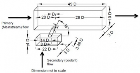
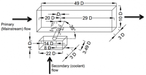
All of the dimensions in Figure 1(a-f) are based on the film-hole diameter D. The delta winglet pair (DWP) has been found in a variety of locations upstream and downstream (see Table 1). The angle of attack is 15o in this case. The CFD (Common Flow down) DWP arrangement was utilized for this study. The grid distribution is shown in Figure 1(g). In the DWP and film-hole regions, finer grids are employed.
Table 1. Details of configuration and position of DWP (VG) (See Figure 1(a-f))
|
|
1 DWP before hole (upstream) |
1 DWP after hole (downstream) |
1 DWP before and after the hole (up and downstream) |
2 DWP after hole (downstream) |
3 DWP after hole (downstream) |
|
Figure 1(a) (Baseline) |
X |
X |
X |
X |
X |
|
Figure 1(b) |
√ |
X |
X |
X |
X |
|
Figure 1(c) |
X |
√ |
X |
X |
X |
|
Figure 1(d) |
X |
X |
√ |
X |
X |
|
Figure 1(e) |
X |
X |
X |
√ |
X |
|
Figure 1(f) |
X |
X |
X |
X |
√ |
(a)
(b)
(c)
(d)
(e)
(f)
(g)
(h)
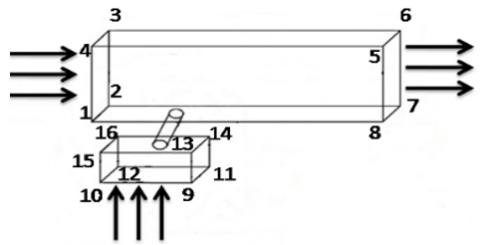
Figure 1. (a)-(f) graphic representation of computational domain and its bottom wall, (g) boundary condition, (h) grid distribution
3.2 Choice of turbulence model
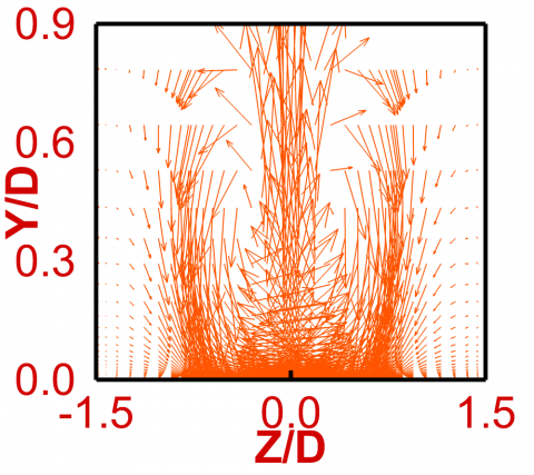
To find the optimum eddy viscosity-based model, researchers looked at several turbulence models (k-$\varepsilon$ standard, k-$\varepsilon$ RNG, k-$\varepsilon$ realizable, k-$\omega$ standard and k-$\omega$ SST). At X/D=10, Figures 2 and 3 show the vector distribution and cross-plane temperature distribution respectively. The k-$\omega$ SST model outperforms all other turbulence models in terms of effectiveness distribution. Under a significant adverse pressure gradient, this model successfully predicts the spreading rate of a jet for a complex flow with rotation, separation, and recirculation. As seen in Figures 2 and 3 among the various turbulence models, the K-$\omega$ SST model performs best due to the lowest effect of jet lift-off & CRVP.
(a)
(b)
(c)
(d)
(e)
Figure 2. Vector distribution for different turbulence models (a) K-epsilon standard, (b) K-epsilon realizable, (c) K-epsilon RNG, (d) K-omega standard and (e) K-omega SST at X/D=10
Figure 3. Cross plane non-dimensional temperature distribution for different turbulence model
(a) K-omega SST, (b) K-omega standard, (c) K-epsilon RNG, (d) K-epsilon relizable and (e) K-epsilon standard at X/D=10
3.3 Governing equation
Three-dimensional flow and heat transmission simulations were performed using a Newtonian fluid with constant physical parameters that were not affected by temperature. Unsteady Reynolds Averaged Navier-Stokes and unsteady energy equations are utilised to take into consideration the impact of turbulence on a large-scale motion. In addition to transport equations such as turbulent kinetic energy and dissipation, the incompressible continuity, momentum, and energy equations must be solved.
In standard form (dimensional form) continuity, momentum and energy equations defined as:
$\frac{\partial {{u}_{i}}}{\partial {{x}_{i}}}=0$ (1)
$\frac{\partial {{u}_{i}}}{\partial t}+\frac{\partial ({{u}_{i}}{{u}_{j}})}{\partial {{x}_{j}}}=-\frac{1}{\rho }\frac{\partial p}{\partial {{x}_{i}}}+\frac{\mu }{\rho }\frac{{{\partial }^{2}}{{u}_{i}}}{\partial {{x}_{j}}^{2}}$ (2)
$\frac{\partial \theta }{\partial t}+\frac{\partial \left( {{u}_{j}}\theta \right)}{\partial {{x}_{j}}}=\frac{k}{\rho {{C}_{p}}}\frac{{{\partial }^{2}}\theta }{\partial {{x}_{j}}^{2}}+\frac{\mu }{\rho {{C}_{p}}}\left[ 2{{\left( \frac{\partial {{u}_{i}}}{\partial {{x}_{i}}} \right)}^{2}}+{{\left( \frac{\partial {{u}_{i}}}{\partial {{x}_{j}}} \right)}^{2}} \right]$ (3)
In dimensionless form continuity, momentum and energy equations defined as:
$\frac{\partial {{u}_{i}}^{*}}{\partial {{x}_{i}}^{*}}=0$ (4)
$\frac{\partial {{u}_{i}}^{*}}{\partial {{t}^{*}}}+\frac{\partial ({{u}_{i}}^{*}{{u}_{j}}^{*})}{\partial {{x}_{j}}^{*}}=-\frac{\partial {{p}^{*}}}{\partial {{x}_{i}}^{*}}+\frac{1}{\operatorname{Re}}\frac{{{\partial }^{2}}{{u}_{i}}^{*}}{\partial {{x}_{j}}{{^{*}}^{^{2}}}}$ (5)
$\frac{\partial {{\theta }^{*}}}{\partial {{t}^{*}}}+\frac{\partial \left( {{u}_{j}}^{*}{{\theta }^{*}} \right)}{\partial {{x}_{j}}^{*}}=\frac{1}{\operatorname{Re}\Pr }\frac{{{\partial }^{2}}{{\theta }^{*}}}{\partial {{x}_{j}}{{^{*}}^{^{2}}}}+\frac{\text{E}}{\operatorname{Re}}\left[ 2{{\left( \frac{\partial {{u}_{i}}^{*}}{\partial {{x}_{i}}^{*}} \right)}^{2}}+{{\left( \frac{\partial {{u}_{i}}^{*}}{\partial {{x}_{j}}^{*}} \right)}^{2}} \right]$ (6)
where,
$\begin{aligned} & \operatorname{Re}=\frac{\rho u_\alpha L}{\mu}=\frac{u_\alpha L}{v}, \operatorname{Pr}=\frac{v}{\alpha}=\left(\frac{\mu}{\rho}\right) /\left(\frac{\mu C_p}{k}\right)=\frac{k}{\rho C_p} \\ & \text { and } \\ & \operatorname{RePr}=\frac{u_\alpha L}{\alpha}=\frac{u_\alpha L}{v} \frac{v}{\alpha}, \mathrm{E}=\frac{u_\alpha{ }^2}{C_p \Delta T}=\frac{u_\alpha{ }^2 / C_p}{\Delta T}\end{aligned}$ (7)
The dimensionless variables are defined:
$\begin{align} & {{u}_{i}}^{*}=\frac{{{u}_{i}}}{{{u}_{\alpha }}},{{u}_{j}}^{*}=\frac{{{u}_{j}}}{{{u}_{\alpha }}},{{x}_{i}}^{*}=\frac{{{x}_{i}}}{L}, \\ & {{p}^{*}}=\frac{p}{\rho {{u}_{\alpha }}^{2}},{{t}^{*}}=t/\left( \frac{L}{{{u}_{\alpha }}} \right),{{\theta }^{*}}=\frac{(T-{{T}_{cf}})}{({{T}_{j}}-{{T}_{cf}})} \\\end{align}$ (8)
Implementing Reynolds decomposition and after that taking time average along with neglecting viscous energy dissipation (when E is small) in energy equation, finally continuity, momentum and energy equations are obtained as:
$\frac{\partial \overline{{{u}_{i}}}}{\partial {{x}_{i}}}=0$ (9)
$\frac{\partial \overline{{{u}_{i}}}}{\partial t}+\frac{\partial (\overline{{{u}_{i}}{{u}_{j}}})}{\partial {{x}_{j}}}=-\frac{\partial \overline{p}}{\partial {{x}_{i}}}+\frac{1}{\operatorname{Re}}\frac{{{\partial }^{2}}\overline{{{u}_{i}}}}{\partial {{x}_{j}}^{2}}+\frac{\partial {{\tau }_{ij}}}{\partial {{x}_{j}}}$ (10)
$\frac{\partial \overline{\theta }}{\partial t}+\frac{\partial \left( \overline{{{u}_{j}}\theta } \right)}{\partial {{x}_{j}}}=\frac{1}{\operatorname{Re}\Pr }\frac{{{\partial }^{2}}\overline{\theta }}{\partial {{x}_{j}}^{2}}+\frac{\partial {{q}_{j}}}{\partial {{x}_{j}}}$ (11)
where, $\tau_{i j}=-\overline{u_i^{\prime} u_j^{\prime}}$ and $q_j=-\overline{u_j^{\prime} \theta^{\prime}}$.
Transport equations can be defined as:
$\frac{\partial }{\partial \text{t}}\left( \rho k \right)+\frac{\partial }{\partial {{x}_{i}}}\left( \rho k{{u}_{i}} \right)=\frac{\partial }{\partial {{x}_{j}}}\left( {{\Gamma }_{k}}\frac{\partial k}{\partial {{x}_{j}}} \right)+{{G}_{k}}-{{Y}_{k}}$ (12)
$\frac{\partial }{\partial \text{t}}\left( \rho \omega \right)+\frac{\partial }{\partial {{x}_{i}}}\left( \rho \omega {{u}_{i}} \right)=\frac{\partial }{\partial {{x}_{j}}}\left( {{\Gamma }_{\omega }}\frac{\partial \omega }{\partial {{x}_{j}}} \right)+{{G}_{\omega }}-{{Y}_{\omega }}+{{D}_{\omega }}$ (13)
The effective diffusivities can be defined as:
${{\Gamma }_{k}}=\mu +\frac{{{\mu }_{t}}}{{{\sigma }_{k}}}$ (14)
${{\Gamma }_{w}}=\mu +\frac{{{\mu }_{t}}}{{{\sigma }_{w}}}$ (15)
Non-dimensionalized length, velocity, time and temperature scale is film hole diameter (D), jet velocity (uj), D/uj and $\theta=\left(T-T_{c f}\right) /\left(T_j-T_{c f}\right)$ respectively. Here Tj and Tcf specifies coolant jet and cross-flow temperature respectively. Here $\tau_{i j}=-\overline{u^{\prime}{ }_l u_j^{\prime}}$ is turbulent stress (Reynolds stress tensor) and $q_j=-\overline{u_j^{\prime} \theta^{\prime}}$ is turbulent heat flux. Turbulent stresses and heat fluxes may be defined through mean quantity with the assist of Boussinesq hypothesis.
${{\tau }_{i}}_{j}=-\overline{u_{i}^{'}u_{j}^{'}}={{\nu }_{t}}\left( \frac{\partial {{\overline{u}}_{i}}}{\partial {{x}_{j}}}+\frac{\partial {{\overline{u}}_{j}}}{\partial {{x}_{i}}} \right)+\frac{2}{3}k{{\delta }_{ij}}$ (16)
$-\left( \overline{{{u}_{i}}'\theta '} \right)={{\alpha }_{t}}\frac{\partial \overline{\theta }}{\partial x{}_{i}}$ (17)
where, suffix t stands for turbulent. νt and αt is the turbulent viscosity and thermal diffusivity. Again, αt may be defined by the ratio of turbulent viscosity to Prandtl number. For the current investigation Prt is taken as 0.85.
${{\alpha }_{t}}=\frac{{{\nu }_{t}}}{{{\Pr }_{t}}}$ (18)
Gk indicates the production of turbulence kinetic energy. Gω delineates about the generation of ω. Γk & Γω specifies effective diffusivity of k & ω respectively. Yk and Yω depicts dissipation of k & ω respectively due to turbulence. Dω depicts cross-diffusion term. ANSYS-FLUENT [23] provides extra information on k-ω SST model. Current investigation used URANS and unsteady energy equation to provide the time-averaged flow and thermal field. Re, Pr represent Reynolds & Pradntl number.
3.4 Boundary condition
In Figure 1(g) and Table 2, the boundary condition has been given. For a blowing ratio (M=ρjuj/ρcfucf) of 1, a numerical research was conducted based on a steady Reynolds number (uαD/ν) of 17000 of free stream velocity (uα=104 m/s) and film cooling hole diameter (D=2.54 mm). The temperature at the primary flow inlet and film-hole output was fixed at 300 and 150 K respectively, for the current investigation. TI is turbulent intensity. 1.75% TI for cross flow, 5.5% TI for jet flow.
Outflow conditions have been applied to the outlet plane. The top surface has a symmetry boundary condition, whereas the bottom wall surface and film hole have no-slip adiabatic wall conditions. The periodic boundary condition is applied in a spanwise direction for the symmetric pair of primary flow domains along with the secondary flow reservoir domain. The wall boundary condition has been provided for the remaining faces. Because the M includes both the density and velocity ratios of the primary and the secondary flow, the ideal averaged coolant ejected velocity for M=0.5 should be around 52 m/s for a fixed primary flow velocity (104 m/s), primary flow domain inlet temperature (300 K), and secondary flow temperature (150 K). The previously described governing equations, as well as these boundary conditions, were solved using the k-omega SST model by ANSYS FLUENT (version 14). ICEMCFD was used to create an unstructured mesh.
Table 2. Boundary conditions (shown in Figure 1(g))
|
Boundaries |
Boundary conditions |
|
1-2-3-4, 9-10-12-11 |
Velocity: Velocity inlet (104 m/s of crossflow, 52 m/s of jet for M=0.5), Temperature: 300 K for cross flow, 150 K for jet flow. |
|
5-6-7-8 |
Outflow |
|
1-4-5-8, 2-3-6-7, 10-15-13-9, 12-16-14-11 |
Periodic |
|
5-6-3-4 |
Symmetry |
|
8-7-2-1 |
Velocity: wall (No slip), Temperature: wall (adiabatic) |
|
9-13-14-11, 10-12-16-15 |
Velocity: wall (No slip), Temperature: wall (adiabatic) |
|
Vortex generator, pipe |
Velocity: wall (No slip), Temperature: wall (adiabatic) |
3.5 Grid independence and convergence analysis
Figure 4. Grid independence study
For unstructured mesh, an analysis of grid independence (Figure 4) was carried out. The near wall mesh is fine enough (Y+≈1) that the laminar sub layer can be resolved. The fine grid (5.3 million nodes), intermediate grid (4.2 million nodes) along with the coarse grid (3.4 million nodes) were both evaluated during this examination. There was a rather minor difference in effectiveness distribution between the coarse, medium and fine grid. It shows that all three grids are getting closer to grid independence. However, the fine grid cases are used in the rest of the analysis. Roache et al. [24] proposed a grid convergence index (GCI) that enables consistent grid convergence reporting based on a grid refinement error estimator evaluated from the idea of generalized Richardson Extrapolation. Three meshes were subjected to a grid convergence analysis.
3.6 Simulation procedure
FLUENT, a commercial computational fluid dynamics code, is used to solve the governing equations (version 14). With the help of ICEMCFD, an unstructured mesh was created. A finer grid has been considered for the close wall region, whereas a coarse grid has been preserved for the far wall zone. For the near-wall treatment, a low Reynolds number model (low RE model) was adopted. The SIMPLE method is used to link pressure and velocity. The second-order upwind approach is used to discretize momentum, energy, turbulent dissipation rate, and turbulent kinetic energy. Convergence criteria are preserved at the order of 10-6 for continuity and momentum equations, whereas it is set to 10-8 for the energy equation. Apart from that, the turbulent kinetic energy dissipation criteria are maintained at the order of 10-4. It's a great concept to measure convergence by looking at residual levels and mass balance and also by monitoring key integrated quantities (static temperature). The convergence was validated by observing the temperature and velocity variations as a function of iteration number and mass balance.
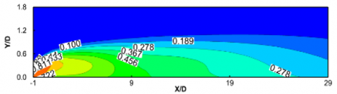
3.7 Validation study
For the validation study, the baseline was examined along with Yao et al. numerical inspection and Kapadia et al experimental inquiry. As shown in Figure 5, the baseline effectiveness distribution is compared to the experimental inquiry of Kapadia et al. From this figure, we can see that the span line effectiveness at X=15 D for baseline is matched with both numerical and experimental studies.
Figure 5. Effectiveness of the span line at X=15D in the baseline validation study
The primary objective of the present study is to investigate the film cooling effectiveness of a gas turbine blade using a vortex generator. The mechanism for the mitigation of CRVP has been discussed. The findings of this study have been discussed including bottom wall film cooling effectiveness, mid-plane temperature, cross-plane temperature and cross-plane vector distribution. The Courant-Friedrichs Levy (CFL) is defined here as (uΔt/Δx). Where maximum velocity in m/s, time step size in s, and minimum grid size in m. The maximum CFL is 1 when Δt is taken to be 10-5 seconds.
4.1 Effect of distance between film cooling hole and vortex generator
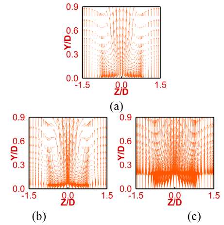
4.1.1 Vector distribution
Figure 6 represents vector distribution at cross-plane for the distance between film cooling hole and the vortex generator. While distance decreases then we have lower strength of CRVP. Also, we have lower vertical distance between vortex core and bottom wall. As a result, we are getting higher effectiveness as depicted by Figure 6(a).
Figure 6. Vector distribution at cross plane (X/D=10) for distance between film cooling and vortex generator. VG located at X/D=(a) 7.89, (b) 9.81 and (c) baseline
4.2 Effect of increase in the vortex generator
Effects of an increase in vortex generator (VG) have been discussed with cross-plane non-dimensional temperature. The RMS (root mean square) value reduces with an increase in VG indicating a reduction in amplitude of fluctuation for increment in VG as compared to baseline.
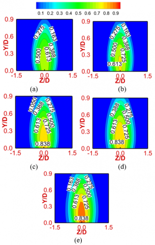
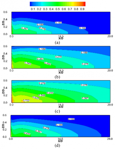
4.2.1 Temperature distribution at cross-sectional plane
Non-dimensional temperature distribution (Figure 7) at the cross-sectional plane (X/D=10) will enlighten that, lower jet lift-off is related to increment in DWP. Reduction in DWP is accountable for higher jet lift-off. Lower jet lift-off is inspected for 3 DWP in Figure 7(a), resulting higher cooling effect by retaining the cold fluid near the bottom wall. Higher aerodynamic loss is observed with an increment of VG. So we can’t increase the number of VG beyond a certain limit.
Figure 7. Non-dimensional temperature distribution for increment in DWP. (a) DWP=3, (b) DWP=2, (c) DWP=1 and (d) baseline at X/D=10
4.3 Effect of vortex generator’s length
Careful examination may express that an increment in effectiveness has been inspected with increments in vortex generator length.
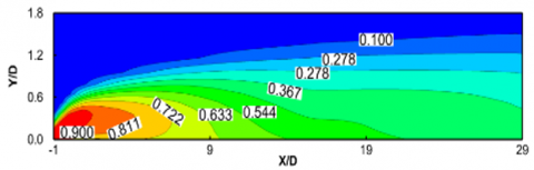
4.3.1 Temperature distribution at mid plane
According to the mid-plane temperature distribution, longer vortex generators result in reduced CRVP strength, which increases bottom wall efficiency (Figure 8).
(a)
(b)
(c)
(d)
(e)
(f)
Figure 8. Non-dimensional temperature distribution at mid plane for different VG length. (a) 6.76 D, (b) 4.94 D, (c) 4.47 D, (d) 4 D, (e) 3.07 D and (f) baseline
4.4 Effect of vortex generator's height
With the enhancement of VG height greater effectiveness is inspected. Usually, we take the height of vortex generator in terms of boundary layer thickness. Here height is taken in terms of film cooling hole diameter. But we cannot go beyond a certain limit due to having pressure drop associated with height.
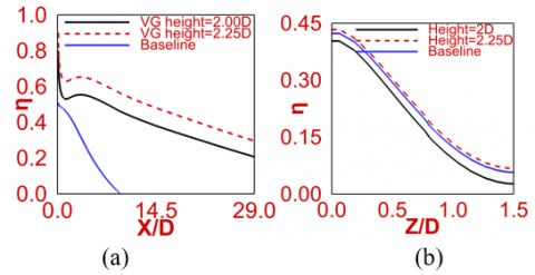
4.4.1 Centerline & span-line effectiveness
Higher & Lower effectiveness has been observed with higher & lower height of vortex generator respectively which may be attributed to jet lift-off as depicted in Figure 9. Lower jet lift-off is responsible for greater effectiveness and lower effectiveness is related with higher jet lift-off.
Figure 9. (a) centerline effectiveness, (b) span line effectiveness at X/D=10 for VG height at 2D, 2.25D
4.5 Effect of Reynolds number
Effect of Reynolds number have been discussed with Temperature distribution at cross-sectional plane.
4.5.1 Temperature distribution at cross-sectional plane
Figure 10 depicts temperature distribution at a cross-sectional plane. At high Re, interaction between primary and secondary flow is more which results in higher jet lift-off. So at Re=20,000, we will obtain high velocity of cold jet flow resulting higher non-dimensional temperature distribution.
Figure 10. Non-dimensional temperature distribution for Re =(a) 15000, (b) 17000, (c) 20000 and (d) baseline at X/D=10
4.6 Effect of turbulent intensity
The effect of turbulent intensity (TI) has been explained with Bottom wall effectiveness distribution (Figure 11).
4.6.1 Bottom wall effectiveness distribution
Figure 11 presents the bottom wall effectiveness distribution. Lower TI depicts lower jet lift-off which allows cold jet flow to remain close to the blade or bottom wall means for lower TI we observe higher bottom wall effectiveness. As higher TI represents higher interaction between cold and hot flow, at TI=5, we obtain the highest bottom wall effectiveness compared to TI=10. At TI=15 we achieve the lowest bottom wall effectiveness.
Figure 11. Bottom wall effectiveness distribution TI=(a) 15, (b) 10, (c) 5 and (d) baseline
In this paper, flow characteristics and film cooling performance were numerically investigated by analyzing effects of blowing ratio and plasma placement of plasma actuation. The primary conclusions are shown as follows.
• Primary vortices (CRVP) are dominant in baseline flow due to the large interaction between the primary and secondary flow. The film cooling effectiveness is reduced due to the strong presence of CRVP, which allows ventilation of hot cross-flow underneath the cold jet.
• Anti-counter-rotating pairs of vortices are generated due to the presence of a delta winglet pair vortex generator. Vortex generator mitigates the detrimental effect of CRVP. With the introduction of DWP, the primary CRVP structures are weakened. A lower level of turbulent mixing between the jet with the cross-flow is observed for the delta winglet pair configuration compared to the baseline case. Lower averaged velocity and attached flow in the near wall region at a lower blowing ratio in DWP configuration indicates lower mixing of the cross-stream flow with the film cooling jet leading to higher film cooling effectiveness.
• Higher film cooling effectiveness is observed for delta winglet pair configuration compared to the baseline case.
• The effect of an increase in VG length and VG height is discussed in this study. The best effectiveness distribution has been attained with an increase in VG length and VG height.
• The consequence of varying the distance between the vortex generator and the film hole is observed. The lowest distance gives better effectiveness.
• Variations of the number of VG are also investigated to explain the effect of DWP. More numbers of VG yield better effectiveness but with pressure loss.
• Among all Re, the lowest Reynolds number will consist best bottom wall effectiveness.
• With the enhancement in turbulent intensity (TI), effectiveness will be decreases.
|
CRVP |
Counter rotating vortex pair |
|
M |
Blowing ratio |
|
ρj |
Density of jet [kg.m-3] |
|
uj |
Jet exit velocity [m.s-1] |
|
ρcf |
Density of cross flow [kg.m-3] |
|
ucf |
Cross flow inlet velocity [m.s-1] |
|
η |
Film cooling effectiveness |
|
Taw |
Adiabatic wall non-dimensional temperature [K] |
|
Tcf |
Cross flow inlet non-dimensional temperature [K] |
|
Tj |
Non-dimensional temperature of jet [K] |
|
VG |
Vortex generator |
|
TV |
Transverse vortices |
|
LV |
Longitudinal vortices |
|
β |
Distance of DWP from leading edge of hole in down as well as upstream direction. |
|
φ |
The angle of attack [O] |
|
DR |
Density ratio |
|
TKE |
Turbulent kinetic energy |
|
LVGs |
Longitudinal vortex generators |
|
WP |
Winglet pair |
|
DWP |
Delta Winglet pair |
|
TI |
Turbulent intensity |
|
DWs |
Delta wings |
|
D |
Diameter of jet [mm] |
|
ν |
Dynamic viscosity [N.s.m-2] |
|
Re |
Reynolds number |
|
X/D |
Ratio of downstream distance from the centre of the film hole to film diameter |
|
Z/D |
Ratio of transverse distance from the centre of the film hole to film diameter |
|
U |
Stream wise velocity [m.s-1] |
|
V |
vertical velocity [m.s-1] |
|
W |
Span wise velocity [m.s-1] |
|
CFU |
Common-flow-up |
|
CFD |
Common-flow-down |
|
Non-dimensional temperature |
(T-Tcf)/(Tj-Tcf) |
[1] Chen, S.P., Chyu, M.K., Shih, T.I.P. (2011). Effects of upstream ramp on the performance of film cooling. International Journal of Thermal Sciences, 50(6): 1085-1094. https://doi.org/10.1016/j.ijthermalsci.2010.10.005
[2] Barigozzi, G., Franchini, G., Perdichizzi, A. (2007). The effect of an upstream ramp on cylindrical and fan-shaped hole film cooling: Part II—adiabatic effectiveness results. In Turbo Expo: Power for Land, Sea, and Air, 47934: 115-123. https://doi.org/10.1115/GT2007-27079
[3] Na, S., Shih, T. (2007). Increasing adiabatic film cooling effectiveness using an upstream ramp. ASME Journal of Heat and Mass Transfer, 129: 464-471. https://doi.org/10.1115/1.2709965
[4] Zhou, W., Hu, H. (2016). Improvements of film cooling effectiveness by using Barchan dune shaped ramps. International Journal of Heat and Mass Transfer, 103: 443-456. https://doi.org/10.1016/j.ijheatmasstransfer.2016.07.066
[5] Rallabandi, A.P., Grizzle, J., Han, J.C. (2011). Effect of upstream step on flat plate film-cooling effectiveness using PSP. ASME Journal of Turbomachinery, 133: 041024. https://doi.org/10.1115/1.4002422
[6] Zhang, F., Wang, X., Li, J. (2016). The effects of upstream steps with unevenly spanwise distributed height on rectangular hole film cooling performance. International Journal of Heat and Mass Transfer, 102: 1209-1221. https://doi.org/10.1016/j.ijheatmasstransfer.2016.07.001
[7] Yousif, H., Kutaeba, J.M., Khishali, AL., Falah, F. (2013). Film cooling experimental investigation for ramped-conical holes geometry. International Journal of Scientific & Engineering Research, 4: 736-745.
[8] Shinn, A., Vanka, S.P. (2011). Numerical simulation of a film-cooling flow with a micro-ramp vortex generator. In 49th AIAA Aerospace Sciences Meeting Including the New Horizons Forum and Aerospace Exposition, p. 767. https://doi.org/10.2514/6.2011-767
[9] van de Wijdeven, T., Katz, J. (2014). Automotive application of vortex generators in ground effect. Journal of Fluids Engineering, 136(2): 1-8. https://doi.org/10.1115/1.4025917
[10] Yao, J., Yao, Y.F. (2011). Computational study of hole shape effect on film cooling performance. Proceedings of the Institution of Mechanical Engineers, Part A: Journal of Power and Energy, 225(4): 505-519. https://doi.org/10.1177/0957650911399013
[11] Kapadia, S., Roy, S., Heidmann, J. (2003). Detached eddy simulation of turbine blade cooling. In 36th AIAA thermophysics conference, p. 3632. https://doi.org/10.2514/6.2003-3632
[12] Katz, J., Morey, F. (2008). Aerodynamics of large-scale vortex generator in ground effect. Journal of Fluids Engineering, 130(7): 071101. https://doi.org/10.1115/1.2948361
[13] Angele, K.P., Grewe, F. (2007). Instantaneous behavior of streamwise vortices for turbulent boundary layer separation control. ASME Journal of Fuids Engineering, 129: 226-235. https://doi.org/10.1115/1.2409327
[14] Park, J., Pagan-Vazquez, A., Alvarado, J.L., Chamorro, L.P., Lux, S.M., Marsh, C.P. (2017). Characterization of tab-induced counter-rotating vortex pair for mixing applications. Journal of Fluids Engineering, 139(3): 031102. https://doi.org/10.1115/1.4034864
[15] Halder, N., Saha, A.K., Panigrahi, P.K. (2021). Enhancement in film cooling effectiveness using delta winglet pair. Journal of Thermal Science and Engineering Applications, 13(5): 051026. https://doi.org/10.1115/1.4049427
[16] Halder, N., Panigrahi, P.K. (2021). Cooling performance of vortex generator. Proceedings of the Institution of Mechanical Engineers, Part A. Journal of Power and Energy, 235: 1619-1638. https://doi.org/10.1177/0957650921993960
[17] Halder, N., Saha, A.K., Panigrahi, P.K. (2017). Influence of delta wing vortex generator on counter rotating vortex pair in film cooling application of gas turbine blade. In Fluid Mechanics and Fluid Power–Contemporary Research: Proceedings of the 5th International and 41st National Conference on FMFP 2014, pp. 95-103. https://doi.org/10.1007/978-81-322-2743-4_10
[18] Bayareh, M., Nourbakhsh, A., Khadivar, M.E. (2018). Numerical simulation of heat transfer over a flat plate with a triangular vortex generator. International Journal of Heat and Technology, 36(4): 1493-1501. https://doi.org/10.18280/ijht.360443
[19] Pourmahmoud, N., Abbaszadeh, M., Rashidzadeh, M. (2016). Numerical simulation of effect of shell heat transfer on the vortex tube performance. International Journal of Heat and Technology, 34(2): 293-301. https://doi.org/10.18280/ijht.340220
[20] Barquín, K., Valencia, A. (2021). Comparison of different fin and tube compact heat exchanger with longitudinal vortex generator in CFU-CFD configurations. International Journal of Heat and Technology, 39(5): 1523-1531. https://doi.org/10.18280/ijht.390514
[21] Syaiful, S., Siwi, A., Utomo, T., Wulandari, Y., Wulandari, R. (2019). Numerical analysis of heat and fluid flow characteristics of airflow inside rectangular channel with presence of perforated concave delta winglet vortex generators. International Journal of Heat and Technology, 37(4): 1059-1070. https://doi.org/10.18280/ijht.370415
[22] Sarifudin, A., Wijayanto, D.S., Widiastuti, I. (2019). Parameters optimization of tube type, pressure, and mass fraction on vortex tube performance using the Taguchi method. International Journal of Heat and Technology, 37(2): 597-604. https://doi.org/10.18280/ijht.370230
[23] ANSYS FLUENT User's Guide. URL: www.pmt.usp.br/academic/martoran/notasmodelosgrad/ANSYS Fluent Users Guide.pdf.
[24] Roache, P.J. (1994). Perspective: A method for uniform reporting of grid refinement studies. ASME Journal of Fluids Engineering, 116(3): 405-413. https://doi.org/10.1115/1.2910291