Saduq Hussein Al-Nasrawei* | Raoof M. Radhi | Mohammed Alhwayzee
© 2022 IIETA. This article is published by IIETA and is licensed under the CC BY 4.0 license (http://creativecommons.org/licenses/by/4.0/).
OPEN ACCESS
Studying industries energy saving is very important prospect for many researchers in the last four decades. In this respect, better process heat transfer can be achieved to improve process operating and capital cost. Thereafter, obtaining higher amount of heat recovery, which will help to reach system optimum heat exchanger network design. Application of Pinch analysis (PA) in our current study, was found to be as an effective method towards economic solution and assessment for all system thermal processes. Whereby, minimizing energy losses, and thus, prediction of maximum energy saving. In addition, application of "Aspen Energy Analyzer (AEA)" simulation software assist our effort to optimize Heat Exchanger Network design (HEN), with various application scenario towards best design. This study represents a "Case study" as a Brayton closed cycle gas turbine power plant in Al-khairat district, which is one of a number of sites used to generate electricity for Iraq national grid. However, the plant original design is open cycle. This study, represent an attempt to apply (PA) in system closed cycle model with the same working conditions. The results predicted, on the contrary of open cycle, that using closed cycle (PA) with temperature difference ∆Tmin can be acceptable with several design propositions. The optimum (∆Tmin = 15℃) were evaluated in the closed cycle system pinch analysis, thereby the maximum Qrec. process that minimize the QHmin & QCmin requirement were identified by the software simulation for the best HEN design. These results were found as Qrec. = 318.330 MW, QHmin = 88.607 MW and QCmin =39.564 MW.
pinch analysis, heat exchanger network, heat recovery, power plant, pinch point
PA method is developed in last four decades, is particularly used in thermal process to predict the maximum energy saving and hot & cold utility requirement. Thereby, optimum design for HEN can be obtained [1].
Such that energy saving can minimize the operating cost in the process [2] and optimum retrofit for HEN [3]. Applying PA IN the WTPS Wanakbori Gujarat power plant to reach an optimum plant design. Starting with ∆Tmin =25℃, so this leads to enhancing the performance of the plant by 47.19% from the 46.78% and decrease the mass of fluid by 0.19 kg/s, which may lead to enhance the plant performance [4, 5]. Applied PA in naphtha unit to reach to optimum HEN design for the plant with ∆Tmin =16℃, there is no improvement in the cost of the process conducted due to decreasing heat and cold loading [6].
Choosing ∆Tmin value of 10℃ [7], PA resulted in good savings of energy for heat utility and cold utility requirement. However, the retrofit of HEN design is important to reach to optimum design for maximum heat recovery Qrec., lead to decrease in CO2 emissions from the plant [8].
The fact that selecting any value of ∆Tmin will be subjected to a tradeoff between energy cost and capital cost. Such calculation and with the help of specific chart to arrive at the proper cost-wise results. The composite curve shows graphically the smallest distance between hot composite curve (HCC) and cold composite curve (CCC), where a positive value of ∆Tmin must be assigned, i.e. for ∆Tmin > 0. Qrec. is connected with the value ∆Tmin so heating and cooling utility are also related to the change with ∆Tmin [9].
The design of HEN and the retrofit for it to arrive to better solution for the plant is depending on the value for temperature difference between hot and cold utility [10]. Several published work [11-13] have investigated operating and capital cost with respect to specific value of ∆Tmin in order to improve heat transfer process and thereby arrive at the best HEN design.
The optimum HEN design is subjected to tradeoff between energy and capital cost and the period of lifetime of HEN [14].
In some designs of HEN is with stream splitting and this method gives a good solution for heat transfer in the process [15]. There are methods to reach to optimum design for HEN with differential evolution to identified the heat loads in the HE [16].
All of the above reviewed research applied PA to improve system performance in terms of operating or capital costs.
However, a selective operating condition was almost a common approach for all researches.
Since (∆Tmin) is a key factor in this respect, then our current work is evaluation attempt for optimum (∆Tmin) graphically to identity maximum Qrec. process that minimize QHmin & QCmin requirement and this we believe is economic achievement.
It is clear from the general theoretical and practical work of the above published studies, PA based on the mathematical and graphical approach is almost always arrive at similar conclusion with respect to energy saving. Therefore, the case study attempt in this paper will be applied to closed power cycle with operating conditions similar to that of Al-khairat gas turbine plant to investigate for possible heat recovery (Qrec.) in all cycle thermal process.
In this respect, the optimum (∆Tmin) should be predicted in order to identify the maximum Qrec. process that minimize the QHmin & QCmin requirement using the software simulation for the best HEN design.
At the end of this Introduction, and in order to achieve the above design objectives, the paper project will be conducted according to the following work program:
2.1 General introduction
PA is developed by linnhoff from Leeds University in his Ph.D study in 1977 for minimizing the energy consumption in a process and reach better heat transfer and heat recovery . He noticed that there is an integration for heat in the process and established the foundation for such analysis, to minimize the total cost of the process connected with the optimum design for heat transfer in the field.
Generally, the PA is based on thermodynamic principles, beginning with the heat and mass balance to identify the hot and cold streams in the process. There by, hot stream need cooling, and the cold stream need heating. Thus integration between them for all the system, is what the PA method is all about [1].
Generally, graphical solution is used in PA problems which comes from two principle diagrams, both of which apply temperature- enthalpy (T-H) relationship. This is symmetrized in Table 1:
Table 1. Compared between CC & GCC
|
Ⅰ- Composite Curve (CC) |
Ⅱ-Grand Composite Curve (GCC) |
|
Figure 1 represent an example of hot & cold (CC) with selected ∆Tmin value. Whereby, minimum heating & cooling utilities (QHmin, QCmin) as well as (Qrec.) can be derived with respect to the assigned ∆Tmin. It should also be noted that at the pinch point, there is no heat flow. |
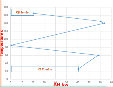
Similarly, Figure 2 represent an example of (GCC) which is plotted from shifted temperature level composite curves. It indicates the difference between the heat available from the process hot streams and the heat required by the process cold streams, relative to the pinch, at a given shifted temperature. Thus, the GCC is a plot of the net heat flow against the shifted (interval)temperature. |
Figure 1. Composite curve
Figure 2. Grand composite curve
2.2 Gas turbine power plant
Gas turbine power plant used to generate electricity for the national grid, constitute three major parts in the open cycle, first the compressor, combustion chamber and finally the turbine, as shown in the illustration of Figure 3 [17].
Figure 3. Gas turbine power plant
Gas power plant is represented thermodynamically by Brayton cycle, and consist of four major parts, namely, compressor; combustion chamber; turbine and finally the cooling water, and with air as working fluid.
The same principles are applied whether the cycle is open or closed type. Whereby, an extra process is included in the closed cycle, by which cooling the working fluid before recycling it back to the compressor, as illustrated schematically in Figure 4 and P-V diagram as in Figure 5 [17]. Therefore, closed cycle system study will be selected with the appropriate mathematical modelling.
Figure 4. Schematic for Gas turbine power plant (closed cycle)
Figure 5. Thermodynamic diagram for Brayton cycle (closed cycle)
2.3 Applied pinch method in the Al-Khairat power plant
Mathematical modelling and PA method were applied to the Al-Khairat closed cycle gas power plant. This site consists of 10 (125MW) electricity generating frame 9Eunits, manufactured by General Electric (GE) industries. As far as this work is concerned, all units were examined, and unit No.3 were chosen for modelling and PA, for its stable working conditions.
The objectives of this study are:
1. calculate Qrec. In the power plant.
2. calculate QHmin in the power plant.
3. calculate QCmin in the power plant.
4. design the HEN for the power plant.
3.1 Theoretical model
Several assumptions were made prior to the theoretical analysis steps. These are:
1. Air is the cycle working fluid.
2. Fuel mass flow is neglected compared high air mass flow.
3. The same (pressure & temperature) in all stages in the power plant.
The mathematical modelling used in the analysis is based on the following:
Ⅰ- heat load in all plant streams, based on the 1th law of thermodynamics is "an expression of the conservation of energy principle" [17]:
$Q-W=H$
But W=0 because there is no mechanical work when it calculates heat load, and heat load can be expressed as:
$Q=\dot{m} \times C p \times \Delta T$ (1)
Ⅱ- efficiency calculation for the power plant is:
$\eta=P / Q a d d$ (2)
where, the efficiency "The fraction of the heat input that is converted to network output is a measure of the performance of a heat engine and is called the thermal efficiency" [17].
Ⅲ- Temperature outlet from combustion chamber "1-2 Isentropic compression (in a compressor), 3-4 Isentropic expansion (in a turbine) and P2= P3 and P4= P1" [17]:
$\frac{\text { To.cc }}{\text { To.tr }}=\left(\frac{\text { Po.cc }}{\text { Po.tr }}\right)^{\frac{(k-1)}{k}}$ where (k=1.4) (3)
Ⅳ- shifted temperature for all streams with ∆Tmin "to allow for the maximum possible amount of heat exchange within each temperature interval. The only modification needed is to ensure that within any interval, hot streams and cold streams are at least ΔTmin apart. This is done by using shifted temperatures" [1].
for hot stream $=$ Thot $-\Delta T \min / 2$ (4)
for cold stream $=T$ cold $+\Delta$ Tmin $/ 2$ (5)
Ⅴ- equation used to calculate heat load in problem table "each interval will have either a net surplus or net deficit of heat as dictated by enthalpy balance, but never both. Knowing the stream population in each interval" [1]:
$\Delta H=(S i-S i+1) \times\left(\sum C P h o t-\sum\right.$ CPcold $)$ (6)
∑CPhot=summation of specific heat in hot streams(kJ/kg.K).
∑CPcold=summation of specific heat in cold streams(kJ/kg.K).
3.2 Theoretical estimation
Acquisition of thermal data were actually obtained from the plant control facilities and from GE documents illustrated Figure 6:
Figure 6. Thermal data for (P and T) in the closed cycle
The specific heat (Cp) is temperature dependent variables, while mass flow rate in all stages is constant (391.2kg/s) for closed cycle. Furthermore, heat load calculation was conducted using Eq. (1). These results are illustrated in the Table 2.
Table 2. Results for heat load in power plant
|
No |
stream |
Ts (℃) |
Tt (℃) |
Cp kJ/kg.K |
$\dot{m}$ kg/s |
CP kW/K |
∆ H MW |
|
1 |
HOT |
907 |
483 |
1.0884 |
391.2 |
425.78 |
180.5 |
|
2 |
HOT |
483 |
32 |
1.0053 |
391.2 |
393.27 |
177.4 |
|
3 |
COLD |
364 |
907 |
1.267 |
391.2 |
495.65 |
269.2 |
|
4 |
COLD |
32 |
364 |
1.061 |
391.2 |
415.06 |
137.8 |
Efficiency evaluation for closed system power plant by the use of Eq. (2),
η=P⁄Qadd=90MW/269.2MW(100)=0.3343=33.43%
From the GE documents, the fuel price is (35.85 ID/lit) & its heating value (LHV) is (42447kJ/kg).
Since ( $\eta$=33.43%), and (LHV=42447kJ/kg), then η=P⁄Qf=90MW/(42447) $\times \dot{m} f \Rightarrow \dot{m} f$=6.348kg/s.
But the actual fuel rate from plant data is (6.833kg/s), so percent saving of mass of fuel is:
6.833 - 6.348/6.833=0.0709=7.098%
Every unit in the plant is fuel consumption (27.5 m3/hr) from GE documents.
Cost of fuel per hour=35.85 ID×1000 liter×27.5 m3/hr=985,875 ID/hr.
Saving cost per hour=985,875×0.0709=69898.53 ID/hr.
Annual cost reduction= $\frac{1}{h r} \cdot \frac{24 h r}{\text { day }} \cdot \frac{\text { 30days }}{\text { month }} \cdot \frac{12 \text { month }}{\text { year }}=8640 \mathrm{hr} / \mathrm{yr}$.
Annual cost reduction $\left(\frac{I D}{y r}\right)=69898.53\left(\frac{8640 h r}{y r}\right)=604\left(10^6\right)$.
Drawing the (T-H) after calculating the ∆H in all streams in the power plant, the results is illustrated in the Figure 7.
In this figure is clear there is region between hot and cold CC which represent ∆Tmin, and therefore, PA can apply on the power plant. Now applying system PA for a range of (5, 10, 15, 20 and 25) ℃ as a specific in turn values of ∆Tmin, following the same procedure each time to evaluate QHmin, QCmin, and Qrec.
First consideration therefore, is (5℃) ∆Tmin, and PA is carried out to draw CC& GCC diagrams according to the following procedure [1]:
Ⅰ. Apply Eqns. (4 & 5) to evaluate shifted temperature for all streams in the closed cycle with choosing ∆Tmin to allow for the maximum possible amount of heat exchange within each temperature interval and this method is help us to know the streams who rejected or received heat by enthalpy balance by using Eq. (6) for each stream as illustrated in Table 3.
Figure 7. Composite curve for closed cycle
Table 3. Shifted temperature for ∆Tmin=5℃
|
No |
stream |
Ts (℃) |
Tt (℃) |
Shifted temp. (℃) |
Shifted temp. (℃) |
|
1 |
HOT |
907 |
483 |
904.5 |
480.5 |
|
2 |
HOT |
483 |
32 |
480.5 |
29.5 |
|
3 |
COLD |
364 |
907 |
366.5 |
909.5 |
|
4 |
COLD |
32 |
364 |
34.5 |
366.5 |
Ⅱ. Apply problem table (temperature intervals) is showing in Figure 8.
Figure 8. Problem table for closed cycle ∆Tmin= 5℃
Ⅲ. Calculate the ∆H for all streams to specified the surplus and deficit streams in the plant by applying Eq. (6) as illustrated in the Table 4:
Table 4. Surplus and deficit for closed cycle in ∆Tmin=5℃
|
|
Interval number |
Si- Si+1 (℃) |
∑CPhot -∑CPcold (kW/℃) |
∆Hi(kW) |
Surplus or deficit |
|
S1=909.5℃
S2=904.5℃
S3=480.5℃
S4=366.5℃
S5=34.5℃
S6= 29.5℃ |
1
2
3
4
5 |
5
424
114
332
5 |
-495.65
- 69.87
- 102.38
-21.79
+393.27 |
-2478.25
-29624.88
-11671.32
-7234.28
+1966.35 |
deficit
deficit
deficit
deficit
surplus |
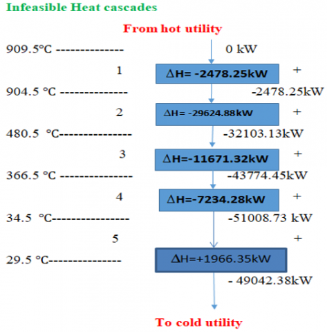
Ⅳ. Do the infeasible heat cascade step using data from Table 4, as illustrated in the Figure 9:
Figure 9. Infeasible heat cascade for ∆Tmin=5℃
Ⅴ. Choosing minimum heat load, in this case is at T=34.5℃ with ∆H=-51008.73 kW. Add this heat load to heat cascade again from hot utility [1].
Ⅵ. Add the value of minimum heat load and start the feasible heat cascade to arrive to temperature where ∆H equal zero. This temperature represents pinch point, as illustrated in the Figure 10:
Figure 10. Feasible heat cascade for ∆Tmin=5℃
So the results for applying pinch method for ∆Tmin=5℃ is:
|
Pinch point (℃) |
Pinch hot point (℃) |
Pinch cold point (℃) |
QHmin MW |
QCmin MW |
Qrec. MW |
|
34.5 |
37 |
32 |
51.008 |
1.966 |
355.929 |
Figure 11. Composite curve for closed system with ∆Tmin=5℃
This analysis procedure is repeated for the other specified temperature (10,15,20 and 25) ℃, and the results is illustrated below in the Table 5.
Table 5. Value of QHmin, QCmin and Qrec. for different ∆Tmin
|
∆Tmin ℃ |
Qrec. MW |
QHmin MW |
QCmin MW |
|
5 |
356.929 |
51.008 |
1.966 |
|
10 |
353.963 |
52.975 |
3.932 |
|
15 |
351.996 |
54.941 |
5.899 |
|
20 |
350.03 |
56.907 |
7.865 |
|
25 |
348.064 |
58.874 |
9.831 |
3.3 Computer program
The computer program used in our work is Aspen Energy Analyzer AEA-Version V11-2019, by but the data obtained from the power plant (T, Cp and inlet & outlet mass flow rates) in all streams in the process is used in this program.
For all the range of ∆Tmin between hot and cold composite curves by applied PA method with theoretical calculations there are Qrec. possible is found and the results for QHmin, QCmin and Qrec. Is shown in Table 6.
Table 6. Value for QHmin, QCmin and Qrec. For different ∆Tmin
|
∆Tmin ℃ |
Qrec. MW |
QHmin MW |
QCmin MW |
|
5 |
356.929 |
51.008 |
1.966 |
|
10 |
353.963 |
52.975 |
3.932 |
|
15 |
351.996 |
54.941 |
5.899 |
|
20 |
350.03 |
56.907 |
7.865 |
|
25 |
348.064 |
58.874 |
9.831 |
By calculating the percent value for each item in the Table 6 the results is:
For ∆Tmin=5℃
Qrec.= 356.929 – 348.064/ 356.929=2.48%
QHmin= 58.874 – 51.008/58.874=13.36%
QCmin=9.831–1.966 /9.831=80%
So the results for all value showing in the Table 7 below:
Table 7. Percent value for Qrec., QHmin and QCmin
|
∆Tmin ℃ |
Qrec. MW % |
QHmin MW% |
QCmin MW % |
|
5 |
0 |
0 |
0 |
|
10 |
0.83 |
3.34 |
20 |
|
15 |
1.38 |
6.68 |
40 |
|
20 |
1.93 |
10.02 |
60 |
|
25 |
2.48 |
13.36 |
80 |
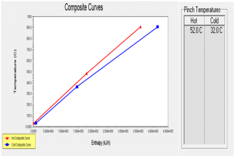
The results for Qrec. & QCmin with ∆Tmin are presented in Figure 12.
Figure 12. Qrec. And QCmin with ∆Tmin
From Figure 12 it's clear that there is cross over between (Qrec. & QCmin) lines at (∆Tmin=15°C), which represent the prediction of the optimum pinch point, and the value of (Qrec.) at this temperature is (351.996 MW).
AEA simulation software is applied to the closed cycle system for a range of ∆Tmin (5, 10, 15, 20 and 25) Because the PA method depends to ∆Tmin between hot and cold utility and by this ∆Tmin reach to optimum design for HEN for the process and this ∆Tmin is different and there is no constant value for it, so by choosing different ∆Tmin and make comparison between them to arrive to better ∆Tmin for the process [1].
The results are shown in the (CC) in Figures 13 and 14.
Figure 13. Thermal data for closed system
The results for AEA simulation software for the range of ∆Tmin between (5, 10, 15, 20 and 25) ℃ is illustrated in the Table 8.
The results for AEA simulation software is showing that there is decrease in Qrec. and increase in QHmin and QCmin with increase ∆Tmin.
Table 8. Qrec., QHmin and QCmin for AEA simulation
|
∆Tmin ℃ |
Qrec. MW |
QHmin MW |
QCmin MW |
|
5 |
356.929 |
51.010 |
1.966 |
|
10 |
353.963 |
52.980 |
3.933 |
|
15 |
351.996 |
54.940 |
5.899 |
|
20 |
350.03 |
56.910 |
7.865 |
|
25 |
348.064 |
58.870 |
9.832 |
(a) For ∆Tmin=5℃
(b) For ∆Tmin=10℃
(c) For ∆Tmin=15℃
(d) For ∆Tmin=20℃
(e) For ∆Tmin=25℃
Figure 14. CC for closed cycle for (a) ∆Tmin=5℃, (b) ∆Tmin=10℃, (c) ∆Tmin=15℃, (d) ∆Tmin=20℃, (e) ∆Tmin=25℃
Thereafter, system GCC are applied for the same temperature range (5, 10, 15, 20 and 25), and the results are shown in the Figure 15.
(a) For ∆Tmin=5℃
(b) For ∆Tmin=10℃
(c) For ∆Tmin=15℃
(d) For ∆Tmin=20℃
(e) For ∆Tmin=25℃
Figure 15. GCC for closed system for (a) ∆Tmin=5℃, (b) ∆Tmin=10℃, (c) ∆Tmin=15℃, (d) ∆Tmin=20℃, (e) ∆Tmin=25℃
The theoretical calculations for closed cycle is illustrated in the Table 9.
The CCs for the system ∆H are presented in Figure 16.
Table 9. Heat loads for power plant
|
No |
stream |
Ts (℃) |
Tt (℃) |
Cp kJ/kg.K |
$\dot{m}$ kg/s |
CP kW/K |
∆ H MW |
|
1 |
HOT |
907 |
483 |
1.0884 |
391.2 |
425.78 |
180.5 |
|
2 |
HOT |
483 |
32 |
1.0053 |
391.2 |
393.27 |
177.4 |
|
3 |
COLD |
364 |
907 |
1.267 |
391.2 |
495.65 |
269.2 |
|
4 |
COLD |
32 |
364 |
1.061 |
391.2 |
415.06 |
137.8 |
Figure 16. CC for closed cycle
So it's clear from the CC that there is a region where PA could be applied at which possible heat transferred between the hot and cold composite curves. Applied the values of heat loads in the AEA simulation program and the results is illustrated in Figure 17.
Figure 17. Composite curve for closed cycle by AEA program
Now applied PA in closed cycle for range of ∆Tmin between (5, 10, 15, 20 and 25) by AEA simulation software and the results is shown in the Figure 18 below.
Figure 18. CC for closed system for (a) ∆Tmin=5℃, (b) ∆Tmin=10℃, (c)∆Tmin=15℃, (d) ∆Tmin=20℃, (e) ∆Tmin=25℃
Theoretical (PA) application and drawing hot and cold CCs for the specified range of ∆Tmin, Qrec. Appeared to be possible. Whereby, the results for Qrec., QHmin and QCmin is shown in Table 10.
Table 10. Qrec., QHmin and QCmin for closed cycle
|
∆Tmin ℃ |
Qrec. MW |
QHmin MW |
QCmin MW |
|
5 |
356.929 |
51.008 |
1.966 |
|
10 |
353.963 |
52.975 |
3.932 |
|
15 |
351.996 |
54.941 |
5.899 |
|
20 |
350.03 |
56.907 |
7.865 |
|
25 |
348.064 |
58.874 |
9.831 |
Validation of the simulation software prediction with theoretical calculations is very important to ensure that such software is reliable, and could be used for different operating conditions, or even for different systems. Both results are presented in Table 11, clearly demonstrate acceptable similarity.
Table 11. Validation for simulation software
|
∆Tmin ℃ |
Qrec. MW |
QHmin MW |
QHmin MW from program |
QCmin MW |
QCmin MW from program |
|
5 |
356.929 |
51.008 |
51.010 |
1.966 |
1.966 |
|
10 |
353.963 |
52.975 |
52.980 |
3.932 |
3.933 |
|
15 |
351.996 |
54.941 |
54.940 |
5.899 |
5.899 |
|
20 |
350.03 |
56.907 |
56.910 |
7.865 |
7.865 |
|
25 |
348.064 |
58.874 |
58.870 |
9.831 |
9.832 |
For all the specified range of ∆Tmin, there are different Qrec. values. Therefore, the correct process Qrec. and the optimal ∆Tmin must be evaluated.
For the optimum ∆Tmin (15℃), it's important to know if the mass of fuel has change or not. Therefore, theoretical calculations will be repeated accordingly to evaluate the mass of fuel.
PA is applied for the calculation of:
Qrec.=Qtr+Q c.w – QCmin -------1
351.996=180.5+ 177.4 – 5.899
Qrec.=Qf+Q comp. – QHmin ---------2
351.996=269.2+137.8 - 54.941
For a comparison purposes, calculate Qf in ∆Tmin=5℃ & 15℃
Ⅰ . with the optimum ∆Tmin=15℃
Qrec.=351.996 MW
Qcomp.=137.8 MW
QHmin=54.941 MW
Qrec.=Qf+Q comp. – QHmin
351.996=Qf+137.8 – 54.941
Ⅱ. calculate Qf in ∆Tmin=5℃ & 15℃
$\checkmark$ for ∆Tmin= 5℃
Qtr+Q c.w – QCmin=Qf+Q comp. – QHmin
180.5+177.4 – 1.966=Qf+137.8 – 51.008
So Q f=269.142 MW
Qf=$\dot{m} f \times \mathrm{C} . \mathrm{V}$
269.142=$\dot{m f} \times$42447
So $\dot{m} f=6.34066 \mathrm{~kg} / \mathrm{s}$
$\checkmark$ for ∆Tmin=15℃
Qtr+Q c.w – QCmin=Qf+Q comp. – QHmin
180.5+177.4 – 5.899=Qf+137.8 – 54.941
So Qf=269.142 MW
Qf=$\dot{m f} \times$ C.V
269.142=$\dot{m f} \times$ 42447
So $\dot{m f}$ =6.34066 kg/s
From the above results, it can be concluded that:
1- The mass flow rate consumption in the different ∆Tmin=5℃ and 15℃ is the same.
2- Design cost decreased due to decrease in Heat Exchanger surface area.
3- Most reference for pinch analysis assume the optimum ∆Tmin between=5 to 25℃.
For optimum temperature difference between hot and cold CC ∆Tmin=15℃ must drawing the HEN design for closed cycle by AEA simulation software and the results is shown below in Figure 19.
The results for Qrec., QHmin and QCmin for all the designs for optimum temperature difference is illustrated in the Tables 12 and 13.
(a) HEN for closed cycle design 1
(b) HEN for closed cycle design 2
(c) HEN for closed cycle design 3
(d) HEN for closed cycle design 4
(e) HEN for closed cycle design 5
(f) HEN for closed cycle design 6
Figure 19. HEN for ∆Tmin=15℃ (a) design1, (b) design 2, (c) design 3, (d) design 4, (e) design 5, (f) design 6
Table 12. Qrec., QHmin and QCmin for six design for HEN
|
∆Tmin ℃ |
Design No. |
Qrec. MW |
QHmin MW |
QCmin MW |
|
15 |
1 |
318.330 |
88.607 |
39.564 |
|
2 |
180.530 |
226.407 |
177.648 |
|
|
3 |
180.530 |
226.407 |
177.648 |
|
|
4 |
318.530 |
88.607 |
39.564 |
|
|
5 |
180.530 |
226.407 |
177.648 |
|
|
6 |
180.530 |
226.407 |
177.648 |
For closed cycle system analysis at optimum temperature difference ∆Tmin= 15℃, there are six HEN design predicted by the software simulation, and from these outcomes, we must identify the better design depending on the values of (Qrec., QHmin and QCmin), and the number HE requirement.
From the Table 12 the (Qrec., QHmin and QCmin) values for each design, and through pinch method philosophy [1], aiming to identify the maximum Qrec. process that minimize the QHmin & QCmin requirement. Design (1 and 4) produced the most attractive results.
From Table 13 the results are presented as number of heat exchanger in each design and is it with or without stream splitting, from which it was concluded that two designs (1 & 4) are the better design. In addition, and with respect to Table 13:
Table 13. Number of HE for each design
|
∆Tmin ℃ |
Design No. |
With stream splitting |
Number of HE for Qrec. |
Number of HE for QHmin |
Number of HE for QCmin |
|
15 |
1 |
Yes |
2 |
2 |
1 |
|
2 |
Yes |
1 |
3 |
1 |
|
|
3 |
No |
2 |
1 |
1 |
|
|
4 |
No |
2 |
1 |
1 |
|
|
5 |
No |
1 |
2 |
1 |
|
|
6 |
No |
2 |
1 |
1 |
Table 14. Characteristics of the selected designs (1) and (4)
|
Design (1) |
Design (4) |
|
With stream splitting |
Without stream splitting |
|
Higher cost of stream splitting design |
Lower cost of none stream splitting design |
|
2 HE in hot utility |
1 HE in hot utility |
Finally, from Table 14 the preferred closed cycle design at ∆Tmin =15℃ is (Design 4) where:
for Qrec.=318.330 MW, QHmin=88.607 MW and QCmin =39.564 MW.
In this study, the investigation for energy saving in the Al-khairat gas turbine power plant is presented to make assessment for the thermal process in the plant to specified the maximum Qrec. and QHmin & QCmin by applied PA method with closed Brayton cycle with the same operating condition in Al-khairat power plant by applied theoretical calculations and with AEA simulation software.
7.1 Conclusions
By calculating ∆H in all the streams in power plant and applied it firstly in the (T-H) diagram and drawing CC to obtained hot and cold composite curve and finally in the AEA simulation software,
1. Can applied PA method in closed cycle because there is heat transfer area between hot and cold CC.
2. Applied range of ∆Tmin between hot and cold composite curve (5, 10, 15, 20 and 25℃).
3. There are Qrec., QHmin and QCmin for each ∆Tmin in the range.
4. There are more than one design for HEN for each ∆Tmin.
5. Choosing the optimum ∆Tmin for closed cycle by predicted it by drawing the values for Qrec. And QCmin and the optimum ∆Tmin is in the 15℃.
6. The values for Qrec., QHmin and QCmin for design four is respectively for Qrec.=318.330 MW , QHmin=88.607 MW and QCmin =39.564 MW.
7. The data for the power plant is obtained by actual site- visit and recorded from the control room facilities. Monitoring such values until it reaches steady level to be considered and recorded for paper analysis. In addition, the methodology depends on step by step PA procedure to reach a specific result which predict the chance to apply PA. Otherwise, choosing another temperature difference between hot and cold composite curves. This is time consuming effort, adding to that careful acquisition of data makes considerable limitation to conduct the test program.
7.2 Recommendations
1. In Iraq the gas turbine power plant used is open Brayton cycle, so the recommendation to used closed Brayton cycle for reasons mentioned in this study.
2. For open cycle to benefit from the exhaust gases from turbine by installed heat recovery steam generation.
3. Future research can involve wide range of temperature difference ∆Tmin up to maybe 50℃ Comparison between such results will obviously allow high accuracy for the specified ∆Tmin processes.
Calculation of process operating and capital cost for process and thus comparison between them with temperature difference ∆Tmin will present better opportunity for optimum heat exchanger network design.
|
CP |
heat capacity, kW.K-1 |
|
|
Cp |
specific heat, kJ. kg-1. K-1 |
|
|
Q,∆H |
heat load, kW |
|
|
P |
power, kW, pressure, bar |
|
|
T |
temperature, K |
|
|
$\dot{\mathrm{m}}$ |
mass flow rate, kg. s-1 |
|
|
Si,Si+1 |
temperature interval, K |
|
|
C.V |
lower heating value, kJ. kg-1 |
|
|
K |
air constant, -- |
|
|
Greek symbols |
||
|
∆ |
difference, -- |
|
|
η |
efficiency, -- |
|
|
∑ |
summation, -- |
|
|
Abbreviations |
||
|
HE, HEN |
Heat exchanger, HE Network |
|
|
QC, QH |
Cold utility, Hot utility |
|
|
M Wt |
Molecular Weight |
|
|
PA |
Pinch Analysis |
|
|
CC |
Composite Curve |
|
|
GCC |
Grand Composite Curve |
|
|
NG |
Natural Gas |
|
|
LDO |
Distillate Gas Oil |
|
|
HFO |
Heavy Fuel Oil |
|
|
GE |
General Electric |
|
|
AEA |
Aspen Energy Analyzer |
|
|
Subscripts |
||
|
s |
supply |
|
|
t |
target |
|
|
1,2,3,4 |
state points |
|
|
e, o |
exit, out |
|
|
i |
inlet |
|
|
cc |
combustion chamber |
|
|
tr |
turbine |
|
|
rec. |
recovery |
|
|
f |
fuel |
|
|
min |
minimum |
|
|
comp. |
compressor |
|
|
c.w |
cooling water |
|
[1] Kemp, I.C., Lim, J.S. (2020). Pinch Analysis for Energy and Carbon Footprint Reduction. Third Edition, Butterworth-Heinemann. https://doi.org/10.1016/C2017-0-01085-6
[2] Goodarzvand-Chegini, F., GhasemiKafrudi, E. (2017). Application of exergy analysis to improve the heat integration efficiency in a hydrocracking process. Energy & Environment, 28(5-6): 564-579. https://doi.org/10.1177%2F0958305X17715767
[3] Čuček, L., Boldyryev, S., Klemeš, J.J., Kravanja, Z., Krajačić, G., Varbanov, P.S., Duić, N. (2019). Approaches for retrofitting heat exchanger networks within processes and Total Sites. Journal of Cleaner Production, 211: 884-894. https://doi.org/10.1016/j.jclepro.2018.11.129
[4] Sunasara, S.R., Makadia, J.J. (2014). Pinch analysis for power plant: A novel approach for increase in efficiency. International Journal of Engineering Research, 3(6): 856-865.
[5] Valiani, S., Tahouni, N., Panjeshahi, M.H. (2017). Optimization of pre-combustion capture for thermal power plants using Pinch Analysis. Energy, 119: 950-960. https://doi.org/10.1016/j.energy.2016.11.046
[6] Manizadeh, A., Entezari, A., Ahmadi, R. (2018). The energy and economic target optimization of a naphtha production unit by implementing energy pinch technology. Case Studies in Thermal Engineering, 12: 396-404. https://doi.org/10.1016/j.csite.2018.06.001
[7] Chauhan, S.S., Khanam, S. (2019). Enhancement of efficiency for steam cycle of thermal power plants using process integration. Energy, 173: 364-373. https://doi.org/10.1016/j.energy.2019.02.084
[8] Mrayed, S., Shams, M.B., Al-Khayyat, M., Alnoaimi, N. (2021). Application of pinch analysis to improve the heat integration efficiency in a crude distillation unit. Cleaner Engineering and Technology, 4: 100168. https://doi.org/10.1016/j.clet.2021.100168
[9] Linnhoff, B., Mason, D.R., Wardle, I. (1979). Understanding heat exchanger networks. Computers & Chemical Engineering, 3(1-4): 295-302. https://doi.org/10.1016/0098-1354(79)80049-6
[10] Li, B.H., Chang, C.T. (2010). Retrofitting heat exchanger networks based on simple pinch analysis. Industrial & Engineering Chemistry Research, 49(8): 3967-3971. https://doi.org/10.1021/ie9016607
[11] Smith, R., Jobson, M., Chen, L. (2010). Recent development in the retrofit of heat exchanger networks. Applied Thermal Engineering, 30(16): 2281-2289. https://doi.org/10.1016/j.applthermaleng.2010.06.006
[12] Wang, Y., Smith, R., Kim, J.K. (2012). Heat exchanger network retrofit optimization involving heat transfer enhancement. Applied Thermal Engineering, 43: 7-13. https://doi.org/10.1016/j.applthermaleng.2012.02.018
[13] Wang, Y., Pan, M., Bulatov, I., Smith, R., Kim, J.K. (2012). Application of intensified heat transfer for the retrofit of heat exchanger network. Applied Energy, 89(1): 45-59. https://doi.org/10.1016/j.apenergy.2011.03.019
[14] Nemet, A., Klemeš, J.J., Kravanja, Z. (2012). Minimisation of a heat exchanger networks' cost over its lifetime. Energy, 45(1): 264-276. https://doi.org/10.1016/j.energy.2012.02.049
[15] Jäschke, J., Skogestad, S. (2014). Optimal operation of heat exchanger networks with stream split: Only temperature measurements are required. Computers & Chemering, 70: 35-49. https://doi.org/10.1016/j.compchemeng.2014.03.020
[16] Thuy, N.T.P., Pendyala, R., Marneni, N. (2014). Heat exchanger network optimization using differential evolution with stream splitting. In Applied Mechanics and Materials, 625: 373-377. https://doi.org/10.4028/www.scientific.net/AMM.625.373
[17] Cengel, Y.A. Boles, M.A. (2005). Thermodynamics: An Engineering Approach. Fifth Edition, McGraw-Hill.