Youssef Tizakast* | Mourad Kaddiri | Mohamed Lamsaadi
© 2021 IIETA. This article is published by IIETA and is licensed under the CC BY 4.0 license (http://creativecommons.org/licenses/by/4.0/).
OPEN ACCESS
The present paper investigates double-diffusive mixed convection inside a horizontal rectangular cavity both numerically using the finite volume method to solve the governing equations and analytically based on the parallel flow approximation developed for the case of shallow enclosures $A \gg 1$. Uniform heat and mass fluxes are applied to the short vertical walls, while the horizontal ones are insulated and impermeable, with top wall sliding from left to right. The results show good agreement between both solutions for a wide range of controlling parameters: Peclet number, Pe, Lewis number, Le, the buoyancy ratio, N, and thermal Rayleigh number, RaT. In order to highlight how the convective regimes influence the effect of controlling parameters on flow and heat and mass transfer characteristics, the parameter RaT/Pe3.0 is established to delineate the zones where natural, mixed, and forced convections dominates the heat and mass transfer. Effects of governing parameters on flow intensity and heat and mass transfer rates are illustrated and discussed in terms of the stream function, $\Psi$, the average Nusselt number, $\overline{N u}$, the average Sherwood number $\overline{S h}$, for the three separated convective regimes.
finite volume method, heat and mass transfer, mixed convection, parallel flow, single lid driven cavity
Double-diffusive convection or thermosolutal convection refers to fluid flows stimulated by buoyancy effects owing to both temperature and concentration gradients, with different rates of diffusion, it’s a subject that continues to attract a lot of attention due to its industrial applications, namely, growth of crystals [1], solar energy systems [2], solidification processes [3] and several others [4-6], showing the great relevance of thermosolutal flows in fluid dynamics. Mixed convection on the other hand, is a result of both buoyancy forces generated by applied temperature and mass gradients, and the shear force, caused by the moving wall.
The majority of mixed convection studies cover flow and heat transfer considering different combinations of cavity configurations and applied thermal gradients [7-13]. Lamarti et al. [14] studied flow heat transfer of two-dimensional Newtonian fluid in a square cavity with a periodically oscillating wall, they conducted that the variation of the Reynolds and Grashof numbers affect strongly the flow structure and the heat transfer depending on the wall moving direction. Furthermore, the variation of Rayleigh number and period of the heated portion influences the Nusselt number on convective structures. Munshi et al. [15] investigated mixed convection in square lid-driven cavity with elliptic obstacle inside and imposed constant heat flux on the lower wall, they concluded that the mixed convection is mainly controlled by Richardson number (Ri), Grashof number (Gr) and Reynolds number (Re).
Driven cavities are present in many industrial applications, flow and heat transfer in solar systems, glass production, food processing, cooling technics to name few, those applications usually combine with mass transfer, showing the importance of studying mixed convection phenomenon introduced by both thermal and mass buoyancy forces. But many of those investigations found in the literature are related to square cavities. Al-Amiri et al. [16] inspected mixed convection due to combined temperature and mass gradients in a square lid-driven cavity. The results showed that by decreasing the Richardson number, Ri, the moving wall shear force dominates, leading to higher heat and mass transfer rates. Kefayati [17] analyzed thermosolutal mixed convection in square enclosure with both horizontal walls moving and filled with shear-thinning fluids. This study has been performed for the related parameters: Richardson number, Lewis number, power-law index, and the buoyancy ratio. Results discuss how the parameters above affects heat and mass transfer. Abbasian Arani et al. [18], Sheremet et al. [19], Kefayati [20] and Hussain et al. [21] also studied mixed convection in single lid-driven square cavities using different boundary conditions with buoyancy forces due to both thermal and mass diffusion.
On the opposite, rectangular cavities attracted less interest, using imposed constant temperatures and concentration. Teamah and El-Maghlany [22] studied numerically the mixed convection in a rectangular cavity with moving upper surface under the combined buoyancy effects of thermal and mass diffusion. They found that decreasing the Richardson number causes the heat and mass transfer rates to increase, for both when the wall moves to the right (assisting flow) or to the left (opposing flow), they stated also that increasing Lewis number enhance mass transfer without affecting the heat transfer, and that both heat and mass transfer rates increase as the absolute value of buoyancy ratio increases. Soufiene Bettaibi et al. [23] investigated numerically thermosolutal mixed convection in rectangular enclosure with moving top wall. They used the multiple relaxation time lattice Boltzmann method to study the flow, while the finite difference method is used to compute the temperature and concentration. this study investigated the accuracy of such model, compared to different numerical methods in the literature, in predicting thermodynamics for mixed convection heat and mass transfer.
In summary, the square cavities are the most studied configurations in literature in the case of double diffusive mixed convection, while few studies that considered rectangular cavities were numerical studies associated with constant temperature and concentration. Hence, thermosolutal mixed convection in a rectangular cavity with moving top wall, occupied with a Newtonian fluid and exposed to heat and mass boundary conditions of Neumann type (i.e., applied heat and mass fluxes) has not been covered yet. The present study aims mainly to simulate thermosolutal mixed convection inside a horizontal rectangular cavity filled with Newtonian fluid and subjected to uniform heat and mass gradients along the short vertical sides, while the horizontal ones are insulated and impermeable, with single lid driven. Both, the numerical solution and the parallel flow approximation based analytical solution, are developed for a wide range of the governing parameters, 1≤RaT≤107, 0.1≤Pe≤500, 10-2≤Le≤102, 10-2≤N≤102, and A=24, while discussing the effect of those parameters on the mixed convection flow and heat and mass transfer rates. Also, the zones highlighting the contribution of natural, forced, and mixed convection to heat and mass transfer rates are defined with respect to the governing parameters.
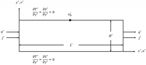
Figure 1 presents the studied configuration with the corresponding boundary conditions. A shallow horizontal rectangular enclosure of height H' and length L', with applied uniform heat and mass fluxes, q' and j', respectively, to the vertical walls, while the horizontal ones are insulated. The cavity is filled with a Newtonian fluid, the top wall is sliding from left to right (assisting flow) with constant velocity $u_{0}^{\prime}$; while the remaining walls are motionless.
For Buoyancy driven flows, the exact governing equations are intractable. Hence, the following frequently used assumptions are adopted, i.e.,
Figure 1. Geometry of the enclosure and coordinates system
Using the stated assumptions, the dimensionless governing equations, representing the conservation of mass (1), momentum (2), (3), energy (4), and concentration (5) written in terms of velocity components (u, v), pressure (p), temperature (T) concentration (S) are as follows:
$\frac{\partial u}{\partial x}+\frac{\partial v}{\partial y}=0$ (1)
$\frac{\partial u}{\partial t}+u \frac{\partial u}{\partial x}+v \frac{\partial u}{\partial y}=-\frac{\partial p}{\partial x}+\operatorname{Pr}\left[\frac{\partial^{2} u}{\partial x^{2}}+\frac{\partial^{2} u}{\partial y^{2}}\right]$ (2)
$\frac{\partial \mathrm{v}}{\partial \mathrm{t}}+\mathrm{u} \frac{\partial \mathrm{v}}{\partial \mathrm{x}}+\mathrm{v} \frac{\partial \mathrm{v}}{\partial \mathrm{y}}=-\frac{\partial \mathrm{p}}{\partial \mathrm{y}}+\operatorname{Pr}\left[\frac{\partial^{2} \mathrm{v}}{\partial \mathrm{x}^{2}}+\frac{\partial^{2} \mathrm{v}}{\partial \mathrm{y}^{2}}\right]$$+\mathrm{Ra}_{\mathrm{T}} \operatorname{Pr}[\mathrm{T}+\mathrm{NS}]$ (3)
$\frac{\partial \mathrm{T}}{\partial \mathrm{t}}+\mathrm{u} \frac{\partial \mathrm{T}}{\partial \mathrm{x}}+\mathrm{v} \frac{\partial \mathrm{T}}{\partial \mathrm{y}}=\left[\frac{\partial^{2} \mathrm{~T}}{\partial \mathrm{x}^{2}}+\frac{\partial^{2} \mathrm{~T}}{\partial \mathrm{y}^{2}}\right]$ (4)
$\frac{\partial \mathrm{S}}{\partial \mathrm{t}}+\mathrm{u} \frac{\partial \mathrm{S}}{\partial \mathrm{x}}+\mathrm{v} \frac{\partial \mathrm{S}}{\partial \mathrm{y}}=\frac{1}{\mathrm{Le}}\left[\frac{\partial^{2} \mathrm{~S}}{\partial \mathrm{x}^{2}}+\frac{\partial^{2} \mathrm{~S}}{\partial \mathrm{y}^{2}}\right]$ (5)
The dimensionless boundary conditions of the problem are:The above equations are obtained by using the following characteristic scales: H', H'2/α, ρ(α2/H'2), α/H', q'H'/λ, j'H'/D corresponding to length, time, pressure, velocity, characteristic temperature, and characteristic concentration, respectively.
$u=v=0$ and $\frac{\partial T}{\partial x}+1=\frac{\partial S}{\partial x}+1=0$ for $x=0$ and $x=A$ (6)
$u=v=0$ and $\frac{\partial T}{\partial y}=\frac{\partial S}{\partial y}=0$ for $y=0 ;$ (7)
$u-P e=v=0$ and $\frac{\partial T}{\partial y}=\frac{\partial S}{\partial y}=0$ for $y=1$ (8)
The stream function, Ψ, is used to study the flow structure:
$u=\frac{\partial \Psi}{\partial y} ; v=-\frac{\partial \Psi}{\partial x}\left(\Psi^{\prime}=0\right.$ on all boundaries $)$ (9)
The governing dimensionless parameters are: the aspect ratio of the enclosure, A, the generalized Prandtl number, Pr, the Peclet number, Pe, the thermal Rayleigh number, RaT, the Lewis number, Le and the buoyancy ratio, N, expressed as:
$\begin{aligned} A &=\frac{L^{\prime}}{H^{\prime}} ; \operatorname{Pr}=\frac{\left(\frac{\mu}{\rho}\right)}{\alpha} ; P e=\frac{u_{0}^{\prime} H^{\prime}}{\alpha} ; \\ \mathrm{Ra}_{\mathrm{T}} &=\frac{\mathrm{g} \beta_{\mathrm{t}} \mathrm{H}^{\prime 4} \mathrm{q}^{\prime}}{\left(\frac{\mu}{\rho}\right) \alpha \lambda} ; \mathrm{Le}=\frac{\alpha}{\mathrm{D}} ; \mathrm{N}=\frac{\beta_{\mathrm{S}} \Delta \mathrm{S}^{*}}{\beta_{\mathrm{T}} \Delta \mathrm{T}^{*}} \end{aligned}$ (10)
where, ρ, g, μ, βT, βS, α and D, are the fluid density, the gravitational acceleration, the dynamic viscosity, the thermal expansion coefficient, the solutal expansion coefficient, the thermal diffusivity and the mass diffusivity, respectively.
Note that:
$P e=\operatorname{RePr}$ and $R a_{T}=G r P r$ (11)
where, Re and Gr are the Reynolds and Grashof numbers, respectively.
The well-known finite volume method and SIMPLER algorithm [26], used to solve the governing Eqns. (1)-(5) with the corresponding boundary conditions (6)-(8) numerically. The temporal terms appearing in (2)-(5) are discretized using a second order backward finite difference scheme. A line-by-line tridiagonal matrix algorithm with relaxation is used in conjunction with iterations to solve the nonlinear discretized equations. The convergence criterion $\sum_{i, j}\left|f_{i, j}^{k+1}+f_{i, j}^{k}\right|<10^{-5} \sum_{i, j}\left|f_{i, j}^{k+1}\right|$ is adopted, where $f_{i, j}^{k}$ is the value of u, v, p, T or S at the kth step. The choice of the grid size was chosen as to have accurate results with a reasonable computation time. Table 1 shows that, for A=24 (value after which the computed entities are invariant to A), a uniform grid size of 341 x 81 is found adequate to simulate accurately the fluid flow, temperature and concentration distribution in the cavity. We used the following initial conditions for the adopted code: u=v=T=S=0.
The local Nusselt and Sherwood numbers describing local heat and mass transfers, respectively, can be defined as:
$N u(y)=\frac{q^{\prime} L^{\prime}}{\lambda \Delta T^{\prime}}=\frac{1}{(\Delta T / A)}$ (12)
$\operatorname{Sh}(y)=\frac{j^{\prime} L^{\prime}}{D \Delta S^{\prime}}=\frac{1}{(\Delta S / A)}$ (13)
where, ΔT=T(0, y)-T(A, y) and ΔS=S(0, y)-S(A, y) represents the local dimensionless temperature and mass difference between the two vertical walls of equations x=0 and x=A, respectively.
The Analytical solution is valid in the core section of the enclosure, and as it will be compared with the numerical solution, and to avoid problems related to edge effects that may result in Eqns. (12)-(13) giving different results, Nu and Sh are evaluated far from the edges of the cavity. Thus, for two infinitesimally adjacent sections, we can express Nu and Sh respectively as:
$\begin{aligned} N u(y) &=\lim _{\delta x \rightarrow 0} \frac{\delta x}{\delta T}=\lim _{\delta x \rightarrow 0} \frac{1}{\left(\frac{\delta T}{\delta x}\right)} \\=&-1 /(\partial T / \partial x)_{x=A / 2} \end{aligned}$ (14)
$\begin{aligned} \operatorname{Sh}(y) &=\lim _{\delta x \rightarrow 0} \frac{\delta x}{\delta S}=\lim _{\delta x \rightarrow 0} \frac{1}{\left(\frac{\delta S}{\delta x}\right)} \\=&-1 /(\partial S / \partial x)_{x=A / 2} \end{aligned}$ (15)
where, δx is the horizontal distance between the two vertical symmetrical sections with respect to the central section at x=A/2.
The average horizontal Nusselt number, representing the overall horizontal heat transfer and the average horizontal Sherwood number, describing the overall horizontal mass transfer can be given respectively as:
$\overline{N u}=\int_{0}^{1} N u(y) d y$ (16)
$\overline{S h}=\int_{0}^{1} \operatorname{Sh}(y) d y$ (17)
Numerical results, displaying streamlines, isotherms, and iso-concentrations, are presented in Figure 2, obtained, for A=24, Le=5, N=1, RaT=105 and different values of Pe. The results show that the flow is parallel to the x-direction, the temperature and concentration exhibit linear stratification in the central region of the cavity with respect to the horizontal direction, independently of the governing parameters. The approximate analytical solution developed next uses the above observations.
Table 1. Grid size choice using $\overline{N u}$ for A=24, Le=5, N=1, RaT=105 and different values of Pe
|
Pe |
Grids |
Analytical Solution |
||||
|
(301,81) |
(321,81) |
(341,81) |
(341,121) |
(361,81) |
||
|
0.1 |
31.601 |
31.658 |
31.689 |
31.660 |
31.722 |
31.401 |
|
1.0 |
31.909 |
31.968 |
32.000 |
31.967 |
32.033 |
31.706 |
|
5.0 |
33.343 |
33.408 |
33.444 |
33.418 |
33.479 |
33.131 |
|
25.0 |
42.4 |
42.506 |
42.572 |
42.555 |
42.633 |
42.143 |
|
50.0 |
59.638 |
59.839 |
59.977 |
59.942 |
60.096 |
59.364 |
|
100.0 |
123.072 |
123.711 |
124.197 |
124.133 |
124.597 |
123.308 |
|
150.0 |
233.249 |
234.808 |
236.045 |
235.906 |
237.045 |
235.538 |
Figure 2. Streamlines (left), isotherms (middle) and isoconcentrations (right) for A=24, Le=5, N=1 and RaT=105 and different Pe values ((a) Pe=0.1, (b) Pe=20 and (c) Pe=100). (Scale not respected)
Based on the observations made on Figure 2, the next simplifications are used:
$u(x, y)=u(y), v(x, y)=0$ and $\Psi(x, y)=\Psi(y)$
$T(x, y)=C_{T}\left(x-\frac{A}{2}\right)+\theta_{T}(y)$
and $S(x, y)=C_{S}\left(x-\frac{A}{2}\right)+\theta_{S}(y)$ (18)
where, CT and CS are respectively, the unknown constant temperature gradient and the unknown constant concentration gradient in x-direction. As a result, the non-dimensional governing equations become:
$\frac{d^{3} u(y)}{d y^{3}}=E R a_{T}$ (19)
$C_{T} u(y)=\frac{d^{2} \theta_{T}(\mathrm{y})}{d y^{2}}$ (20)
$C_{S} u(y)=\frac{1}{L e} \frac{d^{2} \theta_{S}(\mathrm{y})}{d y^{2}}$ (21)
where:
$E=C_{T}+N C_{S}$ (22)
with the following boundary conditions:
$u=\Psi=\frac{d \theta_{T}(y)}{d y}=\frac{d \theta_{S}(y)}{d y}=0$ for $y=0$
$u-P e=\Psi=\frac{d \theta_{T}(y)}{d y}=\frac{d \theta_{S}(y)}{d y}=0$ for $y=1$ (23)
with:
$\int_{0}^{1} u(y) d y=0$ (24)
$\int_{0}^{1} \theta_{T}(y) d y=0$ (25)
$\int_{0}^{1} \theta_{S}(\mathrm{y}) d y=0$ (26)
as return flow, mean temperature and mean concentration conditions, respectively.
Thus, the solutions of (19)-(20), satisfying (23)-(25), are as follows:
$u(y)=\frac{\operatorname{Ra}_{\mathrm{T}} E}{12}\left(2 y^{3}-3 y^{2}+y\right)+P e\left(3 y^{2}-2 y\right)$ (27)
$\begin{aligned} \theta_{T}(\mathrm{y})=& \frac{C_{T} \mathrm{Ra}_{\mathrm{T}} E}{1440}\left(12 y^{5}-30 y^{4}+20 y^{3}-1\right) \\ &+\frac{C_{T} \mathrm{Pe}}{60}\left(15 \mathrm{y}^{4}-20 y^{3}+2\right) \end{aligned}$ (28)
Using Eq. (20) and Eq. (21) and boundary conditions (23), (25) and (26), we can express θS(y) as:
$\theta_{S}(\mathrm{y})=\frac{L e C_{S}}{C_{T}} \theta_{T}(\mathrm{y})$ (29)
The stream function, Ψ(y), is obtained by integrating Eq. (9), using boundary conditions (23) and Eq. (27):
$\Psi(y)=\frac{\mathrm{Ra}_{\mathrm{T}}}{24} E\left(y^{4}-2 y^{3}+y^{2}\right)+P e\left(y^{3}-y^{2}\right)$ (30)
According to [27] the energy and concentration fluxes conditions in the x-direction are:
$\int_{0}^{1}-\frac{\partial \mathrm{T}}{\partial \mathrm{x}} \mathrm{dy}+\int_{0}^{1} \mathrm{u} \mathrm{Tdy}=\int_{0}^{1}-\left(\frac{\partial \mathrm{T}}{\partial \mathrm{x}}\right)_{\mathrm{x}=0 \text { or } \mathrm{x}=\mathrm{A}} \mathrm{dy}$ (31)
$\int_{0}^{1}-\frac{\partial \mathrm{S}}{\partial \mathrm{x}} \mathrm{dy}+\mathrm{Le} \int_{0}^{1} \mathrm{uSdy}=\int_{0}^{1}-\left(\frac{\partial \mathrm{S}}{\partial \mathrm{x}}\right)_{\mathrm{x}=0 \text { or } \mathrm{x}=\mathrm{A}} \mathrm{dy}$ (32)
In the core section of the enclosure, and with conditions (6), Eqns. (31) and (32) becomes:
$C_{T}+1=\int_{0}^{1} u(y) \theta_{T}(\mathrm{y}) d y$ (33)
$C_{S}+1=L e \int_{0}^{1} u(y) \theta_{S}(\mathrm{y}) d y$ (34)
where, replacing u(y), θT(y) and θS(y) by their expressions, gives:
$C_{T}=\frac{1}{-\frac{R a_{T}^{2}}{362,880} E^{2}+\frac{R a_{T} P e}{3360} E-\frac{P e^{2}}{105}-1}$ (35)
$C_{S}=\frac{1}{-\frac{L e^{2} R a_{T}^{2}}{362,880} E^{2}+\frac{L e^{2} \mathrm{Ra}_{\mathrm{T}} P e}{3360} E-\frac{L e^{2} P e^{2}}{105}-1}$ (36)
Finally, using Eq. (22), we obtain the following transcendental equation:
$\frac{\mathrm{Le}^{2} \mathrm{Ra}_{\mathrm{T}}^{4}}{362,880^{2}} \mathrm{E}^{5}-\frac{\mathrm{Le}^{2} \mathrm{Ra}_{\mathrm{T}}^{3} \mathrm{Pe}}{609,638,400} \mathrm{E}^{4}+\mathrm{Ra}_{\mathrm{T}}^{2}\left[\frac{\mathrm{Le}^{2} \mathrm{Pe}^{2}}{19,051,200}\right.$$\left.+\frac{1}{362,880}\left(1+\mathrm{Le}^{2}\right)+\frac{\mathrm{Le}^{2} \mathrm{Pe}^{2}}{11,289,600}\right] \mathrm{E}^{3}+R a_{T}$
$\left[-\frac{\mathrm{Le}^{2} \mathrm{Pe}^{3}}{176,400}-\frac{\mathrm{Pe}}{3,360}\left(1+\mathrm{Le}^{2}\right)+\frac{\mathrm{Ra}_{\mathrm{T}}}{362,880}\left(\mathrm{Le}^{2}+\mathrm{N}\right)\right]$
$\mathrm{E}^{2}+\left[\frac{\mathrm{Le}^{2} \mathrm{Pe}^{4}}{11,025}+\frac{\mathrm{Pe}^{2}}{105}\left(1+\mathrm{Le}^{2}\right)-\frac{\mathrm{Ra}_{\mathrm{T}} \mathrm{Pe}}{3,360}\left(\mathrm{Le}^{2}+\mathrm{N}\right)+1\right]\mathrm{E}+\frac{\mathrm{Pe}^{2}}{105}\left(\mathrm{Le}^{2}+\mathrm{N}\right)+\mathrm{N}+1=0$ (37)
To solve Eq. (37) and obtain the value of E, the Newton-Raphson method is adopted, while for CT and CS values, we refer to Eqns. (35) and (36), for the given values of the governing parameters Le, N, RaT and Pe.
Considering Eqns. (14)-(18), the mean Nusselt and mean Sherwood numbers are constant:
$\overline{N u}=\frac{-1}{C_{T}} ; \overline{S h}=\frac{-1}{C_{S}}$ (38)
In pure natural convection, u(1)=0. In such a situation, the mean Nusselt number and the mean Sherwood number, are as follows:
$\overline{N u}=\frac{R a_{T}^{2}}{362,880} E^{2}+1$ (39)
$\overline{S h}=\frac{L e^{2} R a_{T}^{2}}{362,880} E^{2}+1$ (40)
The case RaT=0 refers to pure forced convection generated only by shear force. Resulting in the following mean Nusselt and mean Sherwood numbers:
$\overline{N u}=\frac{P e^{2}}{105}+1$ (41)
$\overline{S h}=\frac{L e^{2} P e^{2}}{105}+1$ (42)
The analytical solution developed in section 4 based on the parallel flow approximation is valid for enclosures with A>>1. Thus, numerical tests were carried to define the value of A, after which the flow characteristics become invariant to the aspect ratio, also for which the numerical and analytical results agree perfectly for different values of Le, N, Pe and RaT.
The Prandtl number, Pr, affects strongly mixed convection as reported by [28, 29]. While, in contrast, Lamsaadi et al. [30] and Alloui et al. [31] found that when Pr≥1, it doesn’t affect natural convection. In our case, and while referring to Eq. (11), we can reduce the number of controlling parameters, and not need to explicitly use the value of Pr, by using the couple (RaT, Pe), in which Pr is incorporated, instead of (Gr, Re). As a result, the thermosolutal mixed convection flow is governed by the Peclet number, Pe, the thermal Rayleigh number, RaT, the buoyancy ratio, N and the Lewis number, Le, whose effects on the flow structure, heat and mass transfer rates are investigated for natural, mixed and forced convection.
5.1 Determination of the aspect ratio value
In order to find the smallest value of the aspect ratio, A, for which the numerical results are in good agreement with the analytic ones, Figure 3 shows the evolution of with A, for Le=5, N=1, RaT=105 and various values of Pe. It’s obvious that tend to have an asymptotic behavior as A increases. Therefore, a value of A=24 is large enough to achieve results close to the parallel flow approximation results for all considered values of Le, N, RaT, and Pe.
Furthermore, the results introduced in Table 1 validates the analytical approach and the choice of the value A=24 for the numerical code, as both results agree perfectly. In the following sections, the presented figures will confirm such fact in the explored ranges of the governing parameters RaT≤107, Pe≤500, 10-2≤Le≤102 and 10-2≤N≤102.
Figure 3. Evolution of the Nusselt number with the aspect ratio for Le=5, N=1, RaT=105 and different Pe values
5.2 The mixed convection parameter
The goal is to establish the limits for the natural, mixed, and forced convective regimes, the modified Richardson number Gr/Ren (known also as the mixed convection parameter) is widely used for that purpose, as it compares the buoyancy effects to shear one. The exponent depends on the geometry of the cavity and associated boundary conditions.
Note that, setting Le=1, results in heat and mass transfer having same diffusion characteristics, which allows highlighting the implications of mixed convection parameter alone.
To separate the conditions where a convection regime is qualified either as pure (natural or forced) or mixed in a single lid driven rectangular cavity occupied with Newtonian fluid, we calculate the deviation of the heat and mass transfer rates from the values computed in the case of pure convection, if the deviation is less than 5%, the convective regime is considered pure, if not the regime is flagged as mixed. So, to determine the mixed convection parameter, the following ratios are used:
$\varepsilon_{N u_{n}}=\frac{\left|\overline{N u}-\overline{N u_{n}}\right|}{\overline{N u_{n}}} ; \varepsilon_{N u_{f}}=\frac{\left|\overline{N u}-\overline{N u_{f}}\right|}{\overline{N u_{f}}}$ (43)
$\varepsilon_{S h_{n}}=\frac{\left|\overline{S h}-\overline{S h_{n}}\right|}{\overline{S h_{n}}} ; \varepsilon_{S h_{f}}=\frac{\left|\overline{S h}-\overline{S h_{f}}\right|}{\overline{S h_{f}}}$ (44)
where, $\overline{N u_{f}}$ and $\overline{N u_{n}}$ are the average Nusselt numbers for pure forced and natural convections, respectively, $\overline{S h_{f}}$ and $\overline{S h_{n}}$ and are the average Sherwood numbers for pure forced and natural convections, respectively. As explained above, the convective regime is qualified as pure natural / forced when conditions $\varepsilon_{N u_{n}}<5 \%$ and $\varepsilon_{S h_{n}}<5 \% / \varepsilon_{N u_{f}}<5 \%$ and $\varepsilon_{S h_{f}}<5 \%$ are verified. Otherwise, the convective regime is set to be mixed.
Based on Eq. (43) and Eq. (44), the Figure 4 is constructed, the points (log(RaT), log(Pe)) that verify $\left(\varepsilon_{N u_{n}}=5 \%\right.$ and $\left.\quad \varepsilon_{S h_{n}}=5 \%\right)$ and $\left(\varepsilon_{N u_{f}}=5 \%\right.$ and $\left.\varepsilon_{S h_{f}}=5 \%\right)$ are obtained analytically (solid lines) and numerically (symbols), where both solutions agree perfectly. Those points form two parallel straight lines that split the domain of the explored values of RaT and Pe into three zones. The first zone above line (1), where natural convection is predominant. The second zone below line (2), the forced convection is qualified as dominant regime, in between the two lines, the third zone where the mixed convection dominates. The lines (1) and (2) can be correlated in the following relations:
$\frac{R a_{T}}{P e^{3.0}}=\eta_{n}$ and $\frac{R a_{T}}{P e^{3.0}}=\eta_{f}$ (45)
outlining natural and forced convective regime limit, respectively. The values of coefficients ηn and ηfare presented in Table 2 and shown in Figure 4 with dashed lines.
Finally, for the considered cavity configuration and the associated boundary conditions, the mixed convection regime is delimited as follows:
Table 2. Values of ηn and ηf
|
Convection regime |
Natural convection ηn |
Natural convection ηf |
|
|
584.83 |
0.0079 |
$0.0079<\frac{R a_{T}}{P e^{3.0}}<584.83$ (46)
5.3 Dynamical, thermal and solutale fields
Streamlines (left), isotherms (middle) and iso-concentration(right) are shown in Figure 2 for $L e=5, N=1, R a_{T}=10^{5}$ and various values of Pe. As the wall is sliding from left to right, the same direction as the imposed temperature and concentrations gradients, the buoyancy and shear effects work together (assisting flow), causing the flow to be unicellular and clockwise. As for the flow structure, and except the edges of the cavity where the flow experiences a rotation of 180˚, the dynamical field is parallel to the horizontal direction while the thermal and solutale fields are linearly stratified in the x-direction.
On the other hand, for low values of Pe (i.e. when $\frac{R a_{T}}{P e^{3.0}}>\eta_{n}$), the dynamical, thermal and solutale fields are similar to the ones in pure natural convection case, for RaT=105 (Figure 5), where the fields are Centro- symmetric, with horizontal parallelism and a stratification in the core region of the enclosure, which shows that the buoyancy forces dominate the shear one. As increases, the streamlines, isotherms and iso-concentrations become more sensitive to the effect of the moving wall since the Centro-symmetric pattern starts to disappear and the inclinations of the isotherms and iso-concentrations with respect to the y-direction increases, when Pe is large enough (i.e. when $\frac{R a_{T}}{P e^{3.0}}<\eta_{f}$), we end up with patterns similar to the ones in pure forced convection for Pe=100 and Pe=200 (Figure 6), where the streamlines are more packed near the moving wall showing that the flow is powerful in that region, while isotherms and iso-concentrations becomes more tilted and practically linear in the centre of the enclosure, in that case it’s obvious that the shear effect dominates the convection.
It’s worth to note, that as Pe increases, a boundary layer of isothermal and isoconcentrations starts to form next the vertical walls, indicating the heat and mass transfer strengthen in that regions. The layer is more noticeable near the left wall.
Figure 4. Diagram characterizing the convective regimes
Figure 5. Streamlines (left), isotherms (middle) and iso-concentrations (right) for pure natural convection, Le=5, N=1, RaT=105. (Scale not respected)
Figure 6. Streamlines (left), isotherms (middle) and iso-concentrations (right) for pure forced convection: Le=5, N=1 and (a) Pe=100 and (b) Pe=200. (Scale not respected)
Figure 7. Stream function (top), Nusselt number (middle) and Sherwood number (bottom) variations with Pe, for A=24, Le=5, N=1, and different values of RaT
5.4 Effect of Peclet number
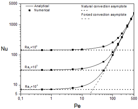
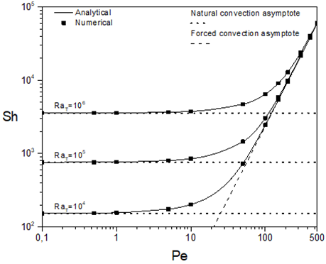
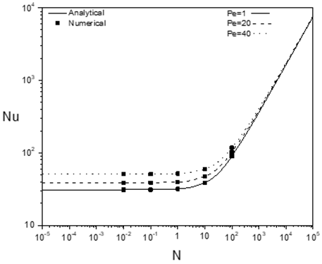
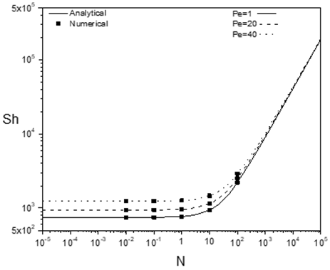
The evolution of $|\Psi c|, \overline{N u}$ and $\overline{S h}$ with the Peclet number, Pe, is presented on Figure 7, for Le=5, N=1 and different values of RaT. For low values of Pe, $\left|\Psi_{c}\right|, \overline{N u}$ and $\overline{S h}$ are invariant to Pe while depending on RaT, plus the results are analogous to the ones obtained in the case of pure natural convection, which indicates that the heat and mass transfer are assured by natural convection, after a certain value of Pe, $\left|\Psi_{c}\right|, \overline{N u}$ and $\overline{S h}$ start to increase slowly due to the contribution of shear effect related to moving wall, this value can be correlated by $\left(\frac{R a}{\eta_{n}}\right)^{1 / 3.0}$, it increases as RaT increases, owing to the well-established effect of Rayleigh number in reinforcing natural convection, thus, delaying the transition from natural regime to mixed one. Finally, as, Pe keeps increasing, the shear effect dominates the buoyancy one until the flow characteristics are governed by forced convection ($\frac{R a_{T}}{P e^{3.0}}<\eta_{f}$) as they increase linearly with Pe, such fact can be confirmed as the results agree with the ones for pure forced convection.
Pure natural convection results are given by the solution of Eq. (39) and Eq. (40) for $\overline{N u}$ and $\overline{S h}$, respectively, and as for forced convection flows, asymptotic limits of the results are defined by the solution of Eq. (41) and Eq. (42) for $\overline{N u}$ and $\overline{S h}$, respectively. Asymptotic limits are indicated by dashed and doted lines.
5.5 Effect of the thermal Rayleigh number
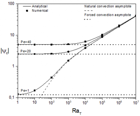
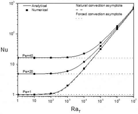
For more understanding of the effect of thermal Rayleigh number, RaT, the variations of $|\Psi c|, \overline{N u}$ and $\overline{S h}$ with this parameter for Le=5, N=1, and various values of Pe, are depicted in. Figure 8. The evolution of $|\Psi c|, \overline{N u}$ and $\overline{S h}$ is similar to that with Peclet number discussed above, as the buoyancy effects and shear one competes. For small values of RaT, $|\Psi c|, \overline{N u}$ and $\overline{S h}$ are invariant as the forced convection is dominating (results agree with the pure forced convection ones), where increasing Pe increases the extent of that range as it strengthens the shear effect, after which they first experiences a slight increase (mixed convection heat transfer), the threshold signaling that change in behavior is defined by (Pe3.0ηf), where forced convection no longer dominates the heat and mass transfer, which agrees with the mixed convection regime limits given by Eq. (46), then after the transition phase, all quantities increase monotonically (dominating natural convection when $\frac{R a_{T}}{p_{e^{3.0}}}>\eta_{n}$), due to the dominating buoyancy effects in promoting the convection. . The dashed lines that indicate the pure forced convection are defined by the solution of Eq. (41) and Eq. (42) for $\overline{N u}$ and $\overline{S h}$, respectively, and as for natural convection, asymptotic limits of the results are defined by the solution of Eq. (39) and Eq. (40) for $\overline{N u}$ and $\overline{S h}$, respectively.
There are two points that deserve mentioning, first, for low values of Pe ($P e \leq 1$), When $R a_{T}$ is small enough ($R a_{T}<10$) the heat and mass transfers are governed by pseudo-diffusion ($\left|\Psi_{c}\right| \leq 10^{-1}, \overline{N u} \approx 1$ and $1<\overline{S h}<2$). Outside this zone, increasing results in increasing $|\Psi c|$ and $\overline{S h}$ without affecting $\overline{N u}$ at first, which increases only when RaT≥100. Second, because Le=5, mass transfer is more important than heat transfer.
Figure 8. Stream function (top), Nusselt number (middle) and Sherwood number (bottom) variations with RaT, for A=24, Le=5, N=1, and different values of Pe
Figure 9. Stream function (top), Nusselt number (middle) and Sherwood number (bottom) variations with Le, for A=24, N=1, RaT=105, and different values of Pe
5.6 Effect of Lewis number
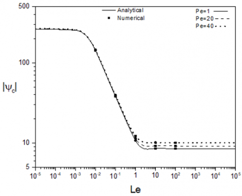
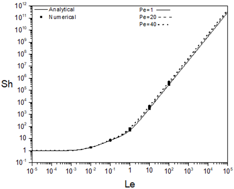
Variations of $\left|\Psi_{c}\right|, \overline{N u}$ and $\overline{S h}$ with Lewis number, Le, are reported in Figure 9 for N=1, RaT=105 and various values of Pe. For low values of Le, the upper plateau for $\left|\Psi_{c}\right|$ and $\overline{N u}$ indicates that thermal convection dominates both thermal conduction and solutal convection, which can be confirmed by the plateau characterized by $\overline{S h} \approx 1$ indicating the diffusive nature of mass transfer. On the other hand, increasing Pe has no effect on flow characteristics, showing that thermal convection also dominates the shear effect induced by driven wall. As Le increases, a descent in the values of $|\Psi c|$ and $\overline{N u}$, while $\overline{S h}$ starts to rise slowly indicates a phase change. Finally, for Le>1, $\overline{S h}$ increases monotonically, this is due to the fact that Sherwood number depends strongly on the Lewis number, while a lower plateau is observed for $|\Psi c|$ and $\overline{N u}$, as the solutal convection with the contribution of the thermal diffusion that increases as Le increases, dominates the thermal convection. Also, the lower plateau shows that increasing Lewis number has no significant outcome on $|\Psi c|$ and $\overline{N u}$, which is expected as the heat transfer is related only to the parameter ($\frac{R a_{T}}{P e^{3.0}}$) that couples natural convection effects with the forced convection ones, which explains the difference in the values of $|\Psi c|$ and $\overline{N u}$ for a fixed value of $\mathrm{Ra}_{\mathrm{T}}$, while varying Pe, where the shear forces obviously affect convection.
Figure 10. Stream function (top), Nusselt number (middle) and Sherwood number (bottom) variations with N, for A=24, Le=5, RaT=105, and different values of Pe
5.7 Effect of the buoyancy ratio
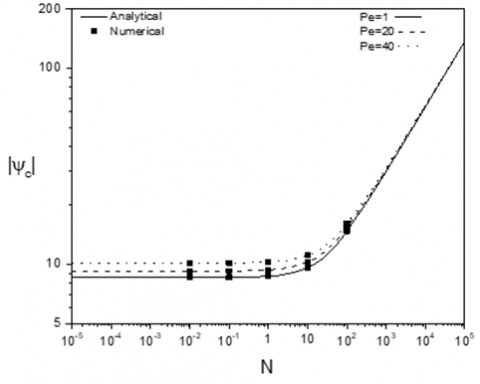
The results of varying $N$ on $\left|\Psi_{c}\right|, \overline{N u}$ and $\overline{S h}$ are reported in Figure 10 for RaT=105, Le=5 and various values of Pe. For aiding flow situation (N>0) discussed here, three convective regimes appear:
for a range of small values of N(N<10), thermal volume force dominates the convection, which results in $\left|\Psi_{c}\right|, \overline{N u}$ and $\overline{S h}$ to be indifferent to changes in value, given the small involvement of solute forces in convection, and only the effect of the moving wall can be seen.
an intermediate regime, for which the increase$\left|\Psi_{c}\right|, \overline{N u}$ and $\overline{S h}$ begins to be seen, the solutal buoyancy force starts to take importance compared to the thermal buoyancy one. As a result, the effect of the moving wall acting in the same direction as the buoyancy forces to enhance convection starts to diminish.
a regime of predominant solutal volume force for which $\left|\Psi_{c}\right|, \overline{N u}$ and $\overline{S h}$ increase in a monotonous and pronounced way with N, thus, the solutal effects are governing the convection, which explains the vanishing effect of the moving wall.
We note that, beyond Le=1000 and N=1000, the numerical code can’t generate stable results.
5.8 Horizontal velocity, temperature and concentration profiles along the y-axis in the central section of the cavity
The horizontal velocity (top), the temperature (centre), and the concentration (bottom) at the core of the enclosure (x=A/2) are shown in Figure 11, for Le=5, N=1, Pe=25 and various values of RaT. When forced convection is dominant, ($R a_{T}<R a_{T c r}$), the illustrated profiles are asymmetric given the fact that horizontal kinematic boundary conditions are of asymmetric nature (only the top wall is moving). For the velocity, as $R a_{T}$ increases, the velocity extremum values augments, as the minimum value becomes more amplified and the maximum value increases as it moves far from the moving wall (y=1), indicating that the flow becomes faster and more intense in that region away from the moving wall, which explains that buoyancy effects dominate convection ($R a_{T}>R a_{T c r}$). The threshold that results in those extremums and indicates that the flow is buoyancy-driven ($R a_{T c r}$), is given by: (see Figure 11).
$R a_{T c r}=\frac{1}{\left[\frac{19}{630}\left(L e^{2}+N\right) P e^{2}+1+N\right.}\left[\frac{1444}{33075} L e^{2} P e^{5}\right.$$\left.+\frac{152}{105}\left(1+L e^{2}\right) P e^{3}+48 P e\right]$ (47)
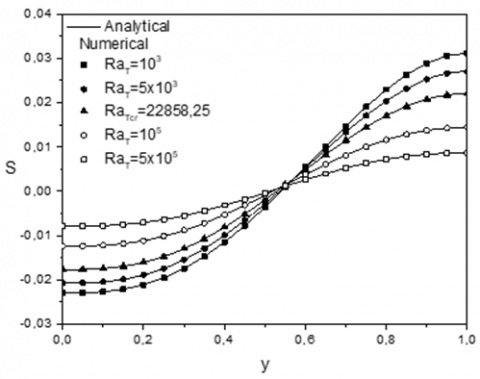
The fact that both shear and buoyancy effects working in the same direction from left to right, results in monocellular clockwise flow, where the velocity is positive on the top region of the cavity while negative on the bottom. As for the temperature and concentration profiles, they also present two zones, the one with positive signs in the top and one with negative signs on the bottom with extremum values that increases as RaT decreases indicating that the flow is losing its intensity as confirmed by the velocity profile and the values of heat and mass transfers that decrease as RaT decreases. For temperature, the clockwise flow makes the top of the cavity warm and the bottom cold by transferring heat from left to right section of the cavity. The concentration exhibits similar phenomenon.
Figure 11. Horizontal velocity (left), temperature (middle) and concentration (right) profiles in the core region of the cavity, along the y-axis for Le=5, N=1, Pe=25 and different values of RaT
Thermosolutal Mixed convection in single lid-driven horizontal rectangular shallow enclosures (A>>1) filled with Newtonian fluid and subjected to uniform heat and mass fluxes applied to the vertical short sides (Neumann type condition) while the long horizontal boundaries are insulated and impermeable is studied numerically and analytically. In the case of shallow enclosures (A≥24), the flow characteristics become indifferent to the increase of the aspect ratio A, which indicates that the governing parameters are reduced to: Lewis number, Le, buoyancy ration, N, Peclet number, Pe, and thermal Rayleigh number, RaT. Numerical solutions, using a finite volume method, are given for wide ranges of governing parameters $\left(10^{-2} \leq L e \leq 10^{2}, 10^{-2} \leq N \leq 10^{2}, 0.1 \leq \mathrm{Pe} \leq\right.$$\left.500,1 \leq \mathrm{Ra}_{\mathrm{T}} \leq 10^{7}\right)$. On the other hand, using the parallel flow approximation valid in the central part of a shallow enclosure, an analytical solution is elaborated, both solutions show good agreement within the explored ranges of the governing parameters. The parameter $\mathrm{Ra}_{\mathrm{T}} / P e^{3.0}$, is found to perfectly outline the natural, forced and mixed convective regimes, where the following boundaries:
$0.0079<\frac{R a_{T}}{P e^{3.0}}<584.83$
delimit the mixed regime for single lid-driven cavity. Whereas, natural and forced convection are found to be dominant outside those limits. The effect of governing parameters on enhancing heat and mass transfer was investigate, where increasing Peclet number results in stronger shear effects, thus increasing heat and mass transfer rates, while increasing Rayleigh number results in a similar effect, but this time due to reinforced buoyancy effects which lead to more active convection. On the other hand, Lewis number affects strongly mass transfer, while no change is noticed on heat transfer. As for increasing buoyancy ratio, it enhances heat and mass transfer, as a beneficial result of dominant solutal buoyancy force.
|
A |
dimensionless aspect ratio of the cavity |
|
$C_{T}$ |
dimensionless temperature gradient in the x-direction |
|
$C_{S}$ |
dimensionless concentration gradient in the x-direction |
|
D |
mass diffusivity $\left(m^{2} / s\right)$ |
|
g |
gravitational acceleration $\left(m^{2} / s\right)$ |
|
Gr |
Grashof number |
|
$H^{\prime}$ |
height of the enclosure $(m)$ |
|
$j^{\prime}$ |
constant mass flux per unit area $\left(\mathrm{kg} / \mathrm{m}^{2} \mathrm{~s}\right)$ |
|
Le |
Lewis number |
|
$L^{\prime}$ |
length of the rectangular enclosure $(m)$ |
|
N |
buoyancy ratio |
|
Nu |
local Nusselt number |
|
$\overline{N u}$ |
mean Nusselt number |
|
Pe |
Peclet number |
|
Pr |
generalized Prandtl number |
|
$q^{\prime}$ |
constant heat flux per unit area $\left(W / m^{2}\right)$ |
|
RaT |
generalized thermal Rayleigh number |
|
Re |
Reynolds number |
|
S |
dimensionless concentration $\left[=\left(S^{\prime}-S_{0}^{\prime}\right) / \Delta S^{*}\right]$ |
|
$\mathrm{S}_{0}^{\prime}$ |
reference concentration $\left(\mathrm{kg} / \mathrm{m}^{3}\right)$ |
|
Sh |
local Sherwood number |
|
$\overline{S h}$ |
mean Sherwood number |
|
T |
dimensionless temperature $\left[=\left(T^{\prime}-T_{0}^{\prime}\right) / \Delta S^{*}\right]$ |
|
$\mathrm{T}_{0}^{\prime}$ |
reference temperature $(K)$ |
|
$\Delta S^{*}$ |
characteristic concentration $\left[=j^{\prime} H^{\prime} / D\right]\left(k g / m^{3}\right)$ |
|
$\Delta T^{*}$ |
characteristic temperature $\left[=q^{\prime} H^{\prime} / \lambda\right](K)$ |
|
$(u, v)$ |
dimensionless axial and vertical velocities $\left[=\left(u^{\prime}, v^{\prime}\right)\left(\alpha / H^{\prime}\right)\right]$ |
|
$(x, y)$ |
dimensionless axial and vertical co-ordinates $\left[=\left(x^{\prime}, y^{\prime}\right) / H^{\prime}\right]$ |
|
Greek symbols |
|
|
$\alpha$ |
thermal diffusivity of fluid $\left(m^{2} / s\right)$ |
|
$\beta_{T}$ |
thermal expansion coefficient of fluid $(1 / K)$ |
|
$\beta_{S}$ |
solutal expansion coefficient of fluid $\left(m^{3} / k g\right)$ |
|
$\lambda$ |
thermal conductivity of fluid $(W / m K)$ |
|
$\mu$ |
dynamic viscosity for a Newtonian fluid $(P a s)$ |
|
$\rho$ |
density of fluid $\left(\mathrm{kg} / \mathrm{m}^{3}\right)$ |
|
$\psi$ |
dimensionless stream function $\left[=\psi^{\prime} / \alpha\right]$ |
|
Superscripts |
|
|
' |
dimensional variable |
[1] Ostrach, S. (1983). Fluid mechanics of crystal growth—the 1982 freeman scholar lecture. ASME Journal of Fluids Engineering, 105: 5-20. https://doi.org/10.1115/1.3240942
[2] Coulter, J.P., Güçeri, S.I. (1987). Laminar and turbulent natural convection in solar energy applications. In Solar Energy Utilization, 303-333. https://doi.org/10.1007/978-94-009-3631-7_14
[3] Nishimura, T., Imoto, T., Miyashita, H. (1994). Occurrence and development of double-diffusive convection during solidification of a binary system. International Journal of Heat and Mass Transfer, 37(10): 1455-1464. https://doi.org/10.1016/0017-9310(94)90147-3
[4] Markham, B.L., Rosenberger, F. (1984). Diffusive-convective vapor transport across horizontal and inclined rectangular enclosures. Journal of Crystal Growth, 67(2): 241-254. https://doi.org/10.1016/0022-0248(84)90184-2
[5] Bergman, T.L., Incropera, F.P., Viskanta, R. (1986). Correlation of mixed layer growth in a double-diffusive, salt-stratified system heated from below. J. Heat Transfer, 108: 206-211. https://doi.org/10.1115/1.3246888
[6] Carlsson, J.O. (1985). Processes in interfacial zones during chemical vapor deposition: Aspects of kinetics, mechanisms, adhesion and substrate atom transport. Thin Solid Films, 130: 261-282. https://doi.org/10.1016/0040-6090(85)90358-X
[7] Waheed, M.A. (2009). Mixed convective heat transfer in rectangular enclosures driven by a continuously moving horizontal plate. Int J Heat Mass Transfer, 52: 5055-63. https://doi.org/10.1016/j.ijheatmasstransfer.2009.05.011
[8] Mekroussi, S., Kherris, S., Mebarki, B., Benchatti, A. (2017). Mixed convection in complicated cavity with non-uniform heating on both sidewalls. Int J Heat Technol, 35(4): 1023-1033. https://doi.org/10.18280/ijht.350439
[9] Nahak, M.P., Triveni, M.K., Panua, R. (2017). Numerical investigation of mixed convection in a lid-driven triangular cavity with a circular cylinder using ANN modeling. International Journal of Heat and Technology, 35(4): 903-918. https://doi.org/10.18280/ijht.350427
[10] Sharif, M.A.R. (2007). Laminar mixed convection in shallow inclined driven cavities with hot moving lid on top and cooled from bottom. Applied Thermal Engineering, 27(5-6): 1036-1042. https://doi.org/10.1016/j.applthermaleng.2006.07.035
[11] Khanafer, K.M., Al-Amiri, A.M., Pop, I. (2007). Numerical simulation of unsteady mixed convection in a driven cavity using an externally excited sliding lid. European Journal of Mechanics-B/Fluids, 26(5): 669-687. https://doi.org/10.1016/j.euromechflu.2006.06.006
[12] Abdelkhalek, M.M. (2008). Mixed convection in a square cavity by a perturbation technique. Comput Mater Sci., 42: 212-219. https://doi.org/10.1016/j.commatsci.2007.07.004
[13] Tiwari, R.K., Das, M.K. (2007). Heat transfer augmentation in a two-sided lid-driven differentially heated square cavity utilizing nanofluids. International Journal of Heat and Mass Transfer, 50(9-10): 2002-2018. https://doi.org/10.1016/j.ijheatmasstransfer.2006.09.034
[14] Lamarti, H., Mahdaoui, M., Bennacer, R., Chahboun, A. (2019). Numerical simulation of mixed convection heat transfer of fluid in a cavity driven by an oscillating lid using lattice Boltzmann method. International Journal of Heat and Mass Transfer, 137: 615-629. https://doi.org/10.1016/j.ijheatmasstransfer.2019.03.057
[15] Munshi, M.J.H., Alim, M.A., Ali, M., Alam, M.S. (2017). A numerical study of mixed convection in square lid-driven with internal elliptic body and constant flux heat source on the bottom wall. Journal of Scientific Research, 9(2): 145-158. https://doi.org/10.3329/jsr.v9i2.29644
[16] Al-Amiri, A.M., Khanafer, K.M., Pop, I. (2007). Numerical simulation of combined thermal and mass transport in a square lid-driven cavity. International Journal of Thermal Sciences, 46(7): 662-671. https://doi.org/10.1016/j.ijthermalsci.2006.10.003
[17] Kefayati, G.R. (2014). Double-diffusive mixed convection of pseudoplastic fluids in a two-sided lid-driven cavity using FDLBM. J Taiwan Inst Chem Eng. https://doi.org/10.1016/j.jtice.2014.05.026
[18] Arani, A.A.A., Ababaei, A., Sheikhzadeh, G.A., Aghaei, A. (2018). Numerical simulation of double-diffusive mixed convection in an enclosure filled with nanofluid using Bejan’s heatlines and masslines. Alexandria Engineering Journal, 57(3): 1287-1300. https://doi.org/10.1016/j.aej.2017.03.034
[19] Sheremet, M.A., Pop, I. (2015). Mixed convection in a lid-driven square cavity filled by a nanofluid: Buongiorno's mathematical model. Applied Mathematics and Computation, 266: 792-808. https://doi.org/10.1016/j.amc.2015.05.145
[20] Kefayati, G.R. (2014). Mesoscopic simulation of magnetic field effect on double-diffusive mixed convection of shear-thinning fluids in a two sided lid-driven cavity. Journal of Molecular Liquids, 198: 413-429. https://doi.org/10.1016/j.molliq.2014.07.024
[21] Hussain, S., Mehmood, K., Sagheer, M., Yamin, M. (2018). Numerical simulation of double diffusive mixed convective nanofluid flow and entropy generation in a square porous enclosure. International Journal of Heat and Mass Transfer, 122: 1283-1297. https://doi.org/10.1016/j.ijheatmasstransfer.2018.02.082
[22] Teamah, M.A., El-Maghlany, W.M. (2010). Numerical simulation of double-diffusive mixed convective flow in rectangular enclosure with insulated moving lid. International Journal of Thermal Sciences, 49(9): 1625-1638. https://doi.org/10.1016/j.ijthermalsci.2010.04.023
[23] Bettaibi, S., Kuznik, F., Sediki, E. (2016). Hybrid LBM-MRT model coupled with finite difference method for double-diffusive mixed convection in rectangular enclosure with insulated moving lid. Physica A: Statistical Mechanics and its Applications, 444: 311-326. https://doi.org/10.1016/j.physa.2015.10.029
[24] Siginer, D.A., Valenzuela-Rendon, A. (2000). On the laminar free convection and stability of grade fluids in enclosures. Int J Heat Mass Transfer, 43: 3391-3405. https://doi.org/10.1016/S0017-9310(99)00357-9
[25] Gray, D.D., Giorgini, A. (1976). The validity of the Boussinesq approximation for liquids and gases. Int J Heat Mass Transfer, 19: 545-51. https://doi.org/10.1016/0017-9310(76)90168-X
[26] Patankar, S.V. (1980). Numerical Heat Transfer and Fluid Flow. Hemisphere, Washington, DC, USA.
[27] Bejan, A. (1983). The boundary layer regime in a porous layer with uniform heat flux from the side. Int. J. Heat Mass Transfer, 26: 1339-1346. https://doi.org/10.1016/S0017-9310(83)80065-9
[28] Karimipour, A., Nezhad, A.H., D'Orazio, A., Shirani, E. (2013). The effects of inclination angle and Prandtl number on the mixed convection in the inclined lid driven cavity using lattice Boltzmann method. Journal of Theoretical and Applied Mechanics, 51(2): 447-462.
[29] Moallemi, M.K., Jang, K.S. (1992). Prandtl number effects on laminar mixed convection heat transfer in a lid-driven cavity. International Journal of Heat and Mass Transfer, 35(8): 1881-1892. https://doi.org/10.1016/0017-9310(92)90191-T
[30] Lamsaadi, M., Naimi, M., Hasnaoui, M. (2006). Natural convection heat transfer in shallow horizontal rectangular enclosures uniformly heated from the side and filled with non-Newtonian power law fluids. Energy Convers Manage, 47: 2535-2551. https://doi.org/10.1016/j.enconman.2005.10.028
[31] Alloui, I., Benmoussa, H., Vasseur, P. (2010). Soret and thermosolutal effects on natural convection in a shallow cavity filled with a binary mixture. International Journal of Heat and Fluid Flow, 31(2): 191-200. https://doi.org/10.1016/j.ijheatfluidflow.2009.11.008