Krishnandan Verma* | Debozani Borgohain | Bishwaram Sharma
© 2021 IIETA. This article is published by IIETA and is licensed under the CC BY 4.0 license (http://creativecommons.org/licenses/by/4.0/).
OPEN ACCESS
The present study investigates numerically MHD flow near the stagnation point of micropolar fluid through a shrinking sheet containing nanoparticles under the influence of chemical reaction and external heat. The study is an attempt to investigate the flow behaviour of micropolar nanofluid because of its importance in heat transfer process in industries as well as cooling systems. The governing equations are converted to nonlinear ordinary differential equations by implementing similarity transformations. Numerical results are investigated in the form of figures and tables by using MATLAB built in solver bvp4c for various dimensionless parameters. The impacts of external heat parameter on temperature and chemical reaction factor on concentration of the nanofluid are illustrated in the form of graphs. It is observed that the temperature of the nanofluid and nanoparticle volume distributions increase when Biot number attain larger values. Rise in Thermophoretic parameter increases the nanoparticles concentration in the boundary layer. Numerical data are presented for Nusselt number and Sherwood number.
MHD, external heat, micropolar nanofluid, shrinking sheet, chemical reaction, bvp4c
Problems related to fluid flow over shrinking or stretching surfaces have struck the eyes of modern researchers because of its numerous applications in industries like food manufacturing, production of paper, polymer extrusion etc. Micropolar fluid is a type of Non-Newtonian fluid which can explain the intrinsic motion and deformation of many materials like suspended particles, polycrystalline materials etc., that Newtonian fluids are not able to do so. Microploar fluid consists of suspended rigid small body particles in viscous medium and its model was first introduced by C. A. Eringen [1]. Unlike Newtonian fluid, micropolar fluid provides greater resistance to motion of the fluid and is used in industries for its various applications like lubricant fluids, colloidal solutions, biological fluids etc. Sakiadis [2] was the first investigator to explore the boundary layer flow problem past a continuous extending surface. Uddin [3] investigated two dimensional, steady micropolar fluid flow through an inclined surface with varying electric conductivity in porous medium. Haq et al. [4] investigated numerically the flow problem of micropolar nanofluid with radiation and buoyancy effects. In fact, many researchers under many different situations studied the flow characteristics of micropolar fluids [5-7].
The stagnation point flow of fluids basically non- Newtonian fluid has attracted the attention of research workers from a very long time because of many important applications in submarines, missiles designing etc. Heimenz [8] used the numerical Keller box method to study MHD boundary layer fluid flow considering viscous dissipation and external heat effects near the stagnation point. Kamal et al. [9] obtained dual solutions for stagnation point MHD flow of nanofluid over stretching/shinking sheet. Haq et al. [10] investigated MHD stagnation point flow with thermal radiation where he explored the zero normal flux condition near the wall of the sheet. Ghaffari et al. [11] adopted the numerical Chebyshev Spectral Newton iterative scheme to study the flow behaviour of viscoelastic fluid over a stretching surface with oblique stagnation point considering radiation.
Nanofluid is a fluid containing nanoparticles suspended in a base fluid, which have quite high thermal conductivity. The applications of nanofluid are seen in petroleum engineering, medical therapy etc., because it is chemically stable and shows enhanced heat transfer rate. Hsiao [12] studied heat and mass transfer flow problem with nanoparticles, convection, magnetic field, viscous dissipation and radiation. Tiwari and Das [13] studied numerically the flow due to nanofluid in a heated lid-driven square cavity with mixed convection and uniform heat flux and found that the convection is due to the buoyancy forces. Mansur and Ishak [14] studied numerically nanofluid flow past an extended/shrinking plate under convective boundary conditions. Hayat et al. [15] investigated the flow problem with convective boundary conditions of Maxwell nanofluid under the existence of magnetic effects. Hayat et al. [16] investigated Casson nanofluid model past an extending surface with radiation, external heat, and chemical effects. Vasantakumari and Pondy [17] analysed the two dimensional viscous incompressible nanofluid flow through an inclined surface with heat generation or absorption effects using Homotopy Analysis Method. Siddik et al. [18] analysed micropolar nanofluid with thermal, radiative and solutal convection conditions above a shrinking surface at the stagnation point. Many researchers studied fluid flow problems with nanoparticles, heat generation /absorption and chemical reaction on different geometry, which can be looked in the literature [19-21].
From the above listed reviews of literature and the growing popularity of micropolar nanofluid in engineering and industrial sector, we are inspired to analyse numerically the flow problem of micropolar nanofluid for stagnation point MHD flow over a shrinking sheet with heat source and chemical reaction. The numerical solution is obtained by using Matlab’s build in solver bvp4c.
Consider the stagnation point two dimensional flow of a laminar, incompressible micropolar nanofluid flowing in the direction normal to a shrinking sheet. The sheet is at a higher temperature and the fluid is electrically conducting. A stationary magnetic field of strength B0 is applied in the transverse direction. The electric field is also taken into account but due to zero polarization voltage, it is equal to zero. The shrinking sheet is in contact with hot fluid of temperature Tf due to which the sheet gets heated up. The free stream temperature is T∞ and free stream concentration of the fluid is C∞. Joule heating and Viscous dissipation effects are neglected. The governing equations of the problem are:
$\frac{\partial u}{\partial x}+\frac{\partial v}{\partial y}=0$ (1)
$\rho\left(u \frac{\partial u}{\partial x}+v \frac{\partial u}{\partial y}\right)=-\frac{\partial p}{\partial x}+(\mu+\kappa) \frac{\partial^{2} u}{\partial y^{2}}+\kappa \frac{\partial \vartheta^{*}}{\partial y}+$$\sigma_{e} B_{0}^{2}(U-u)$ (2)
$\rho j\left(u \frac{\partial \vartheta^{*}}{\partial x}+v \frac{\partial \vartheta^{*}}{\partial y}\right)=\gamma \frac{\partial^{2} \vartheta^{*}}{\partial y^{2}}-\kappa\left(2 \vartheta^{*}+\frac{\partial u}{\partial y}\right)$ (3)
$u \frac{\partial T}{\partial x}+v \frac{\partial T}{\partial y}=\alpha \frac{\partial^{2} T}{\partial y^{2}}+\tau\left(D_{B} \frac{\partial C}{\partial y} \frac{\partial T}{\partial y}+\frac{D_{T}}{T_{\infty}}\left(\frac{\partial T}{\partial y}\right)^{2}\right)+$$\frac{16 \sigma T_{\infty}^{3}}{3 k^{*}} \frac{\partial^{2} T}{\partial y^{2}}+\frac{Q}{\rho c_{p}}\left(T-T_{\infty}\right)$ (4)
$u \frac{\partial C}{\partial x}+v \frac{\partial C}{\partial y}=D_{B} \frac{\partial^{2} C}{\partial y^{2}}+\frac{D_{T}}{T_{\infty}} \frac{\partial^{2} T}{\partial y^{2}}-K_{1}^{*}\left(C-C_{\infty}\right)$ (5)
where, $\vartheta^{*}=\left(\vartheta_{1}, \vartheta_{2}, \vartheta_{3}\right) \text { and } \tau=\frac{(\rho c)_{p}}{(\rho c)_{f}}$.
Boundary conditions are:
$u(x, 0)=b x, v(x, 0)=0, \vartheta^{*}(x, 0)=0$,
$-\kappa \frac{\partial T}{\partial \nu}=h_{1}\left(T_{f}-T\right),-D_{B} \frac{\partial C}{\partial v}=h_{2}\left(C_{f}-C\right)$,
$u(x, \infty)=U=a x, \vartheta^{*}(x, \infty)=0, T(x, \infty)=T_{\infty}$,
$C(x, \infty)=C_{\infty}$. (6)
where, b<0 denotes rate of shrinking of the sheet and the heat and mass transfer coefficients are h1 and h2 respectively.
The similarity transformations used to make the Eqns. (1)-(5) dimensionless are as follows:
$u=a x f^{\prime}(\eta), v=-\sqrt{a \vartheta} f(\eta), \vartheta_{2}=-a \sqrt{\frac{a}{\vartheta}} x g(\eta)$,
$p=p_{0}-\frac{\rho a^{2}}{2}\left(x^{2}+y^{2}\right), \eta=y \sqrt{\frac{a}{\vartheta}}, \theta(\eta)=\frac{T-T_{\infty}}{T_{f}-T_{\infty}}$, (7)
$\phi(\eta)=\frac{C-C_{\infty}}{C_{f}-C_{\infty}}$
where, p0 represents stagnation pressure.
Dimensionless forms of Eqns. (1)-(5) by using (7) are as follows:
$\left(1+R_{1}\right) f^{\prime \prime \prime}+f f^{\prime \prime}-f^{\prime 2}+M^{2}\left(1-f^{\prime}\right)-R_{1} g^{\prime}+1=0$ (8)
$C_{1} g^{\prime \prime}+R_{1} A_{1}\left(f^{\prime \prime}-2 g\right)+f g^{\prime}-f^{\prime} g=0$ (9)
$\left(1+\frac{4}{3} R d\right) \theta^{\prime \prime}+\operatorname{Prf} \theta^{\prime}+\operatorname{Pr} N_{b} \phi^{\prime} \theta^{\prime}+\operatorname{Pr} N_{t} \theta^{\prime 2}+\operatorname{Pr} \lambda \theta=0$ (10)
$\phi^{\prime \prime}+S c f \phi^{\prime}+\left(\frac{N_{t}}{N_{b}}\right) \theta^{\prime \prime}-K_{1} S c \phi=0$ (11)
where, $M=\sqrt{\frac{\sigma_{e} B_{0}^{2}}{\rho a}}, R_{1}=\frac{\kappa}{\mu}, C_{1}=\frac{\gamma}{\mu j}, A_{1}=\frac{\mu}{\rho j a}$, $R d=\frac{4 \sigma T_{\infty}^{3}}{k k^{*}}, P r=\frac{\mu c_{p}}{k}, S c=\frac{\vartheta}{D_{B}}, \lambda=\frac{Q}{a \rho c_{p}}, K_{1}=\frac{K_{1}^{*}}{a}$, $N_{b}=\frac{(\rho c)_{p} D_{B}\left(C_{f}-C_{\infty}\right)}{(\rho c)_{f} \vartheta} \text { and } N_{t}=\frac{(\rho c)_{p} D_{T}\left(T_{f}-T_{\infty}\right)}{(\rho c)_{f} T_{\infty}}$.
The boundary conditions (6) in dimensionless form take the form as follows:
$f(0)=0, f^{\prime}(0)=N, g(0)=0, \theta^{\prime}(0)=-B_{i 1}(1-\theta(0))$,
$\phi^{\prime}(0)=-B_{i 2}(1-\phi(0))$,
$f^{\prime}(\infty)=1, g(\infty)=0, \theta(\infty)=0, \phi(\infty)=0$. (12)
where, $N=-\frac{b}{a}, B_{i 1}=\frac{h_{1}}{\kappa} \sqrt{\frac{\vartheta}{a}} \text { and } B_{i 2}=-\frac{h_{2}}{D_{B}} \sqrt{\frac{\vartheta}{a}}$.
Couple stress and local skin-friction in non-dimensional form are:
$M_{w}=\mu u_{w}\left(1+\frac{R_{1}}{2}\right) g^{\prime}(0)$ (13)
$C_{f} R e_{x}^{1 / 2}=\left(1+R_{1}\right) f^{\prime \prime}(0)$ (14)
Nusselt number,
$N u_{x} R e_{x}^{-1 / 2}=-\left(1+\frac{4}{3} R d\right) \theta^{\prime}(0)$ (15)
Sherwood number,
$S h_{x} R e_{x}^{-1 / 2}=-\phi^{\prime}(0)$ (16)
where, $R e_{x}=\frac{u_{w} x}{\vartheta}$.
Eqns. (8)-(11) with respect to the boundary restriction (12) are solved numerically using Matlab’s built in solver bvp4c which implements a collocation method to obtain the solution of boundary value problems. Eqns. (8)-(11) are converted to set of first order differential equations.
$f=y_{1}, f^{\prime}=y_{1}^{\prime}=y_{2}, f^{\prime \prime}=y_{2}^{\prime}=y_{3}$,
$f^{\prime \prime \prime}=y_{3}^{\prime}=\frac{-y_{1} y_{3}+y_{2}^{2}-M^{2}\left(1-y_{2}\right)+R_{1} y_{5}-1}{\left(1+R_{1}\right)}$,
$g=y_{4}, g^{\prime}=y_{4}^{\prime}=y_{5}$,
$g^{\prime \prime}=y_{5}^{\prime}=\frac{-R_{1} A_{1}\left(y_{3}-2 y_{4}\right)-y_{1} y_{5}+y_{2} y_{4}}{C_{1}}$,
$\theta=y_{6}, \theta^{\prime}=y_{6}^{\prime}=y_{7}$,
$\theta^{\prime \prime}=y_{7}^{\prime}=\frac{-\operatorname{Pry}_{1} y_{7}-\operatorname{Pr} N b y_{9} y_{7}-\operatorname{Pr\lambda} y_{6}-\operatorname{Pr} N t y_{7}^{2}}{\left(1+\frac{4}{3} R d\right)}$,
$\phi=y_{8}, \phi^{\prime}=y_{8}^{\prime}=y_{9}, \phi^{\prime \prime}=y_{9}^{\prime}=\frac{A}{\left(1+\frac{4}{3} R d\right)}$,
where, $A=-\left(1+\frac{4}{3} R d\right) S c y_{1} y_{9}+\left(1+\frac{4}{3} R d\right) K_{1} S c y_{8}+\left(\frac{N t}{N b}\right) \operatorname{Pr} y_{1} y_{7}+N t \operatorname{Pr} y_{9} y_{7}+\left(\frac{N t}{N b}\right) \operatorname{Pr} \lambda y_{6}+\left(\frac{N t^{2}}{N b}\right) \operatorname{Pry}_{7}^{2}$.
The boundary conditions are given by: $y_{1}(0), y_{2}(0)=N, y_{4}(0), y_{7}(0)=-B_{i 1}\left(1-y_{6}(0)\right)$, $y_{9}(0)=-B_{i 2}\left(1-y_{8}(0)\right)$, $y_{2}(\infty)=1, y_{4}(\infty), y_{6}(\infty), y_{8}(\infty)$.
The numerical results obtained are illustrated by figures and tables. The dimensionless physical parameters for which the numerical results have been obtained are $\lambda, K_{1}, B_{i 1}, N_{t}, N_{b}, B_{i 2}, M, R d \text { and } N$.The results are obtained by setting the values of the parameters $C_{1}=0.1, A_{1}=\operatorname{Pr}=0.2, S c=B_{i 1}=B_{i 2}=0.3, M=0.5, R d=0.4, N_{t}=N_{b}=0.4, N=-0.5, R_{1}=2.0, \lambda=0.1$ and $K_{1}=1$ and the value of one parameter is changed at each time for obtaining the graphs.
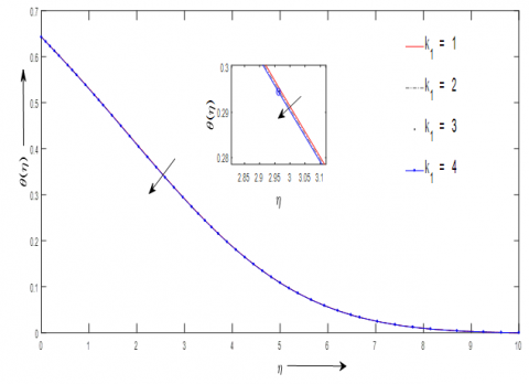
Figure 1 depicts the impact of heat generation parameter $\lambda$ on temperature profiles. The increasing values of λ enhances the temperature as it generates heat in the flow field, which increases the temperature inside the thermal boundary layer. Figure 2 reveals that the value of ϕ(η) decreases exponentially with the increasing values of η. It also reveals that ϕ(η) decreases with increase in the values of λ. Thus we can conclude that the concentration of the nanoparticles decreases as we go away in the normal direction from the shrinking sheet. This concentration also decreases with increase in the values of external heat source and with the decrease in the values of the kinematic viscosity.
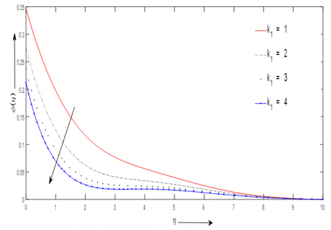
Figure 3 illustrates the impact of chemical reaction parameter K1 on temperature of the micropolar nanofluid. It is spotted from the figure that the larger values of chemical reaction parameter contributes to the decrease in the temperature. Figure 4 represents the influence of K1 on concentration of the nanoparticles. The increment in the values of K1 reduces the nanoparticles concentration as well as concentration boundary layer thickness. Chemical reaction parameter is inversely proportional to the constant $a$. Therefore lower values of a will reduce the nanoparticles concentration in the boundary layer.
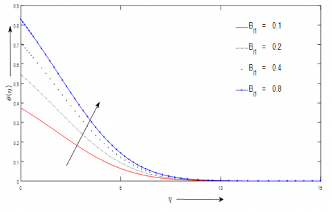
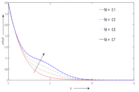
Figure 5 depicts the consequence of heat transfer Biot number $B_{i 1}$ on temperature profiles. It is spotted from the figure that the increasing values of $B_{i 1}$ increase the temperature profile. The increment in temperature is seen because the convective heat transfer at the surface of the sheet increases the thermal boundary layer thickness. Moreover Biot number and heat transfer coefficient are related directly to each other and hence greater values of Biot number enhance heat transfer which ultimately higher the temperature. Figure 6 reflects the distribution of nanoparticles concentration $\phi(\eta)$ due to thermophoretic parameter $N_{t}$. The figure shows that concentration profile is enhanced with higher values of $N_{t}$. Thermophoresis is the process by which tiny particles move to a colder region from the hotter one i.e. $N_{t}$ is dependent on temperature gradient of the surrounding. The thermophoresis force is increased by the larger values of thermophoretic parameter in the region near the boundary layer which ultimately leads to a larger nanoparticles volume concentration.
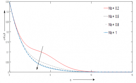
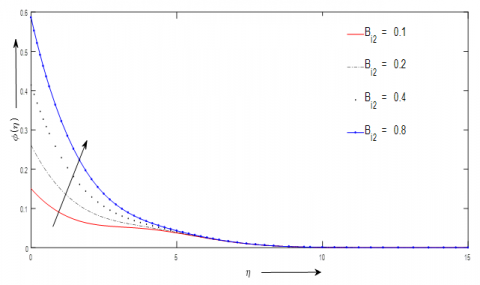
The impact on nanoparticles concentration distribution $\phi(\eta)$ due to Brownian motion parameter $N_{b}$ is shown in Figure 7. The increasing values of $N_{b}$ decrease the boundary layer thickness, thereby decreasing the concentration profile. The impact of $N_{b}$ on nanoparticle volume fraction is just opposite to $N_{t}$. Figure 8 represents the impact of mass transfer Biot number Bi2 on concentration profiles. From the figure, it is observed that the concentration profile is enhanced with the increasing value of Bi2. Concentration increases because the thermal boundary layer thickness increases with the increase in the value of Bi2.
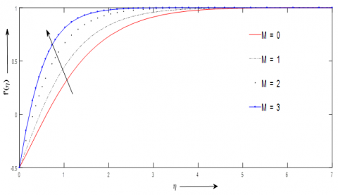
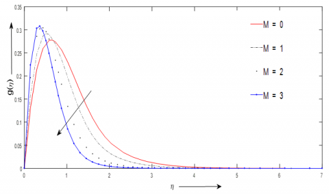
Figure 9 and Figure 10 reflects the change in velocity and microrotation profiles due to magnetic parameter M. Lorentz force is produced due to the magnetic field and it provides resistance to the momentum of the particles of fluid. It is seen from Figure 9 that the velocity boundary layer shifts towards the sheet due to the Lorentz force. In Figure 10 it is seen that the microrotation profiles increases upto $\eta=0.5$ and after that it decreases asymptotically till the end of the boundary layer with the increasing values of magnetic parameter. The decrement in the microrotation profiles is basically due to the Lorentz force which hinders the fluid velocity.
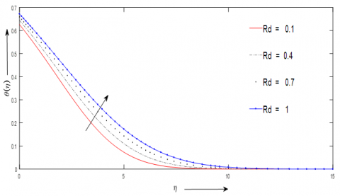
Figure 11 reveals that the change in temperature profile due to radiation parameter $R d$. The temperature and its associated boundary layer thickness increase for the larger values of radiation parameter. The thermal radiation provides heat into the fluid due to which the temperature and the thickness of the boundary layer are enhanced.
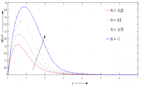
The influence of Shrinking parameter, N on velocity and microrotations profiles are depicted by Figure 12 and Figure 13 respectively. It is observed from Figure 12 that the velocity profiles decrease with the increasing values of Shrinking parameter. In fact, a reversed fluid flow is noticed for the increased magnitude of N near the sheet’s surface. From Figure 13 it is seen that the enhanced values of N increases the microrotation profiles.
Table 1 and Table 2 are computed to check the numerical accuracy of the current work with the previous work of Siddiq et al. [18]. Numerical values of couple stress and skin friction coefficient are obtained for $M \text { and } N$ when the value of the parameters are taken as $C_{1}=0.1, R d=0.4, A_{1}=P r=0.2, S c=0.3, B_{i 1}=B_{i 2}=0.3, N_{t}=N_{b}=0.4, \lambda=0 \text { and } K_{1}=0$. The present results show good match with the results obtained by Siddiq et al. [18].
Table 3 shows the influence of $C_{1}=0.1, N_{t}=0.4, A_{1}=0.2, M=0.5, S c=0.3, N_{b}=0.4, B_{i 2}=0.3, N=-0.5, R_{1}=2.0, \lambda=0.1 \text { and } K_{1}=1$ on Nusselt number for $P r, R d \text { and } B_{i 1}$. It is seen that Nusselt number is enhanced for larger values of $P r, R d \text { and } B_{i 1}$.
Table 4 shows the influence of the parameters $S c, N_{t}, N_{b} \text { and } B_{i 2}$ on Sherwood number for $C_{1}=0.1, A_{1}=\operatorname{Pr}=0.2, B_{i 1}=0.3, M=0.5, R d=0.4, N-0.5, R_{1}=2.0, \lambda=0.1 \text { and } K_{1}=1$. Sherwood number increases for increasing values of $B_{i} \text { and } S c$. A very small increment in Sherwood number is observed for larger values of $N_{t}$. For $0.2 \leq N_{b} \leq 0.8$ the values of Sherwood number remain the same but when $N_{b}=1$ an increment in Sherwood number is noticed.
Table 1. Comparison of the current outcomes of skin-friction coefficient for several values of M, N with Siddiq at al. [18]
|
$M$ |
$-N$ |
$\left(1+R_{1}\right) f^{\prime \prime}(0)$ Siddiq et al. [18] |
$\left(1+R_{1}\right) f^{\prime \prime}(0)$ Present result |
|
0 1 2 3 0.5 0.5 0.5 0.5 |
0.5 0.5 0.5 0.5 0.25 0.5 0.75 1 |
0.77352 1.12096 1.81906 2.61387 0.81718 0.87217 0.87054 0.78922 |
0.7735 1.1210 1.8191 2.6139 0.8172 0.8722 0.8705 0.7892 |
Table 2. Comparison of the current outcomes of couple stress for several values of M, N with Siddiq at al. [18]
|
$M$ |
$-N$ |
$g^{\prime}(0)$ Siddiq et al. [18] |
$g^{\prime}(0)$ Present result |
|
0 1 2 3 0.5 0.5 0.5 0.5 |
0.5 0.5 0.5 0.5 0.25 0.5 0.75 1 |
1.10512 1.38129 1.81669 2.19515 1.00758 1.18905 1.33185 1.38322 |
1.1051 1.3813 1.8168 2.1449 1.0076 1.1891 1.3319 1.3833 |
Table 3. Data collection of local Nusselt number for several values of $B_{i 1}, \operatorname{Pr} \text { and } R d$
|
$B_{i 1}$ |
$\operatorname{Pr}$ |
$R d$ |
$-\left(1+\frac{4}{3} R d\right) \theta^{\prime}(0)$ |
|
0.1 0.2 0.4 0.8 0.3 0.3 0.3 0.3 0.3 0.3 0.3 0.3 |
0.2 0.2 0.2 0.2 0.1 0.2 0.4 0.7 0.2 0.2 0.2 0.2 |
0.4 0.4 0.4 0.4 0.4 0.4 0.4 0.4 0.1 0.4 0.7 1.0 |
0.0626 0.0908 0.1171 0.1368 0.0926 0.1068 0.1181 0.1231 0.0926 0.1068 0.1181 0.3356 |
Table 4. Data collection of Sherwood number for several values of $B_{i 2}, S c, N_{t} \text { and } N_{b}$
|
$B_{i 2}$ |
$S c$ |
$N_{t}$ |
$N_{b}$ |
$-\phi^{\prime}(0)$ |
|
0.1 0.2 0.4 0.8 0.3 0.3 0.3 0.3 0.3 0.3 0.3 0.3 0.3 0.3 0.3 0.3 |
0.3 0.3 0.3 0.3 0.1 0.2 0.3 0.5 0.3 0.3 0.3 0.3 0.3 0.3 0.3 0.3 |
0.4 0.4 0.4 0.4 0.4 0.4 0.4 0.4 0.1 0.3 0.5 0.7 0.4 0.4 0.4 0.4 |
0.4 0.4 0.4 0.4 0.4 0.4 0.4 0.4 0.4 0.4 0.4 0.4 0.2 0.5 0.8 1.0 |
0.0850 0.1477 0.2343 0.3314 0.1546 0.1818 0.1960 0.2120 0.1957 0.1959 0.1962 0.1967 0.1960 0.1960 0.1960 0.1961 |
Figure 1. Variation of $\theta(\eta) \text { due to } \lambda$
Figure 2. Variation of $\phi(\eta) \text { due to } \lambda$
Figure 3. Variation of $\theta(\eta) \text { due to } K_{1}$
Figure 4. Variation of $\phi(\eta) \text { due to } K_{1}$
Figure 5. Variation of $\theta(\eta) \text { due to } B_{i 1}$
Figure 6. Variation of $\phi(\eta) \text { due to } N_{t}$
Figure 7. Variation of $\phi(\eta) \text { due to } N_{b}$
Figure 8. Variation of $\phi(\eta) \text { due to } B_{i 2}$
Figure 9. Variation of $f^{\prime}(\eta)$ due to M
Figure 10. Variation of $g(\eta)$ due to M
Figure 11. Variation of $\theta(\eta) \text { due to } R d$
Figure 12. Variation of $f^{\prime}(\eta) \text { due to } \mathrm{N}$
Figure 13. Variation $g(\eta)$ due to N
The current study is an attempt to analyse the flow behaviour of micropolar fluid containing nanoparticles through a shrinking sheet because of its importance in heat transfer process in industries as well as cooling systems. The outcomes derived during the study are:
I am very much thankful to the reviewers for their valuable suggestions as it helped us to improve the quality of the research paper.
|
a, b |
constants, $s^{-1}$ |
|
$A_{1}$ |
microinertia density parameter |
|
$B_{0}$ |
magnetic field strength, $W b \cdot m^{-2}$ |
|
$B_{i 1}$ |
heat transfer Biot number |
|
$B_{i 2}$ |
mass transfer Biot number |
|
C |
fluid concentration |
|
$C_{1}$ |
dimensionless spin gradient viscosity, |
|
$C_{f}$ |
surface volume fraction |
|
$C_{\infty}$ |
ambient fluid concentration |
|
$c_{p}$ |
specific heat capacity, $J . k g^{-1} . K^{-1}$ |
|
T |
fluid temperature, K |
|
$T_{f}$ |
sheet temperature, K |
|
$T_{\infty}$ |
ambient fluid temperature, K |
|
$D_{B}$ |
Brownian diffusion coefficient |
|
$D_{T}$ |
thermophoretic diffusion coefficient |
|
j |
microinertia density, $m^{-2}$ |
|
$\mathcal{K}$ |
vortex viscosity, $\mathrm{Kg} \cdot \mathrm{m}^{-1} \cdot \mathrm{s}^{-1}$ |
|
k* |
absorption coefficient |
|
k |
thermal conductivity, $W \cdot m^{-1} \cdot K^{-1}$ |
|
$K_{1}^{*}$ |
rate of chemical reaction |
|
$K_{1}$ |
chemical reaction parameter |
|
M |
magnetic field parameter |
|
N |
shrinking parameter |
|
$p$ |
pressure, $P a$ |
|
$p_{0}$ |
stagnation pressure, $P a$ |
|
$N_{b}$ |
Brownian motion parameter |
|
$N_{t}$ |
Thermophoretic parameter |
|
$\operatorname{Pr}$ |
Prandtl number |
|
Q |
heat generation/absorption rate, $W \cdot m^{-3}$ |
|
$R_{1}$ |
vortex viscosity parameter |
|
$R d$ |
thermal radiation parameter |
|
$S c$ |
Schmidt number |
|
$T_{f}$ |
sheet temperature, K |
|
$T_{\infty}$ |
ambient temperature, K |
|
$u$ |
velocity component in x direction, $m \cdot s^{-1}$ |
|
$v$ |
velocity component in y direction, $m \cdot s^{-1}$ |
|
$\operatorname{Re}_{x}$ |
local Reynolds number |
|
U |
velocity away from the sheet, $m \cdot s^{-1}$ |
|
Greek symbols |
|
|
$\alpha$ |
thermal diffusivity of the fluid, $m^{2} s^{-1}$ |
|
$\gamma$ |
spin gradient viscosity, $\mathrm{kg} \cdot \mathrm{m} \cdot \mathrm{s}^{-1}$ |
|
$\mu$ |
dynamic viscosity, $N . s . m^{-2}$ |
|
$\rho$ |
fluid density, $K g \cdot m^{-3}$ |
|
$\vartheta$ |
kinematic viscosity, $m^{2} \cdot s^{-1}$ |
|
$\lambda$ |
heat generation/absorption parameter |
|
$\sigma_{e}$ |
electrical conductivity of the fluid |
|
$\sigma$ |
Stephens Boltzmann constant |
|
$\theta$ |
dimensionless temperature |
|
$\phi$ |
dimensionless nanoparticles concentration |
|
$\vartheta^{*}$ |
microrotation, $s^{-1}$ |
|
$\tau$ |
ratio of nanoparticle heat capacity and base fluid heat capacity |
|
Subscripts |
|
|
p |
nanoparticle |
|
f |
base fluid |
[1] Eringen, A.C. (1964). Simple microfluids. International Journal of Engineering Science, 2(2): 205-217. https://doi.org/10.1016/0020-7225(64)90005-9
[2] Sakiadis, B.C. (1960). Boundary layer behaviour on continuous solid surfaces. 1. Boundary Layer Equations for Two-dimensional and Axisymmetric Flow, 2: 26-28.
[3] Uddin, M. (2011). Convective flow of micropolar fluids along an inclined flat plate with variable electric conductivity and uniform surface heat flux. DIU Journal of Science and Technology, 6: 69-79. http://hdl.handle.net/20.500.11948/536
[4] Haq, R.U., Nadeem, S., Akbar, N.S., Khan, Z.H. (2014). Buoyancy and radiation effect on stagnation point flow of micropolar nanofluid along a vertically convective stretching surface. IEEE Transactions on Nanotechnology, 14(1): 42-50. https://doi.org/10.1109/TNANO.2014.2363684
[5] Ashraf, M., Bashir, S. (2012). Numerical simulation of MHD stagnation point flow and heat transfer of a micropolar fluid towards a heated shrinking sheet. International Journal for Numerical Methods in Fluids, 69(2): 384-398.
[6] Turkyilmazoglu, M. (2016). Flow of a micropolar fluid due to a porous stretching sheet and heat transfer. International Journal of Non-Linear Mechanics, 83: 59-64. https://doi.org/10.1016/j.ijnonlinmec.2016.04.004
[7] Sheremet, M.A., Pop, I., Ishak, A. (2017). Time-dependent natural convection of micropolar fluid in a wavy triangular cavity. International Journal of Heat and Mass Transfer, 105: 610-622. https://doi.org/10.1016/j.ijheatmasstransfer.2016.09.044
[8] Hiemenz, K. (1911). Die Grenzschicht an einem in den gleichformigen Flussigkeitsstrom eingetauchten geraden Kreiszylinder. Dinglers Polytech. J., 326: 321-324.
[9] Rehman, F.U., Nadeem, S., Rehman, H.U., Haq, R.U. (2018). Thermophysical analysis for three-dimensional MHD stagnation-point flow of nano-material influenced by an exponential stretching surface. Results in Physics, 8: 316-323. https://doi.org/10.1016/j.rinp.2017.12.026
[10] Haq, R.U., Nadeem, S., Khan, Z.H., Akbar, N.S. (2015). Thermal radiation and slip effects on MHD stagnation point flow of nanofluid over a stretching sheet. Physica E: Low-dimensional Systems and Nanostructures, 65: 17-23. https://doi.org/10.1016/j.physe.2014.07.013
[11] Ghaffari, A., Javed, T., Labropulu, F. (2017). Oblique stagnation point flow of a non-Newtonian nanofluid over stretching surface with radiation: A numerical study. Thermal Science, 21(5): 2139-2153. https://doi.org/10.2298/TSCI150411163G
[12] Hsiao, K.L. (2014). Nanofluid flow with multimedia physical features for conjugate mixed convection and radiation. Computers & Fluids, 104: 1-8.
[13] Tiwari, R.K., Das, M.K. (2007). Heat transfer augmentation in a two-sided lid-driven differentially heated square cavity utilizing nanofluids. International Journal of heat and Mass transfer, 50(9-10): 2002-2018. https://doi.org/10.1016/j.ijheatmasstransfer.2006.09.034
[14] Mansur, S., Ishak, A. (2013). The flow and heat transfer of a nanofluid past a stretching/ shrinking sheet with a convective boundary condition. Abstract and Applied Analysis, 1-9. https://doi.org/10.1155/2013/350647
[15] Hayat, T., Muhammad, T., Shehzad, S.A., Chen, G.Q., Abbas, I.A. (2015). Interaction of magnetic field in flow of Maxwell nanofluid with convective effect. Journal of Magnetism and Magnetic Materials, 389: 48-55. https://doi.org/10.1016/j.jmmm.2015.04.019
[16] Hayat, T., Ashraf, M.B., Shehzad, S.A., Alsaedi, A. (2015). Mixed convection flow of casson nanofluid over a stretching sheet with convectively heated chemical reaction and heat source/sink. Journal of Applied Fluid Mechanics, 8(4): 803-813.
[17] Vasanthakumari, R., Pondy, P. (2018). Mixed convection of silver and titanium dioxide nanofluids along inclined stretching sheet in presence of MHD with heat generation and suction effect. Mathematical Modelling of Engineering Problems, 5(2): 123-129. https://doi.org/10.18280/mmep.050210
[18] Siddiq, M.K., Rauf, A., Shehzad, S.A., Abbasi, F.M., Meraj, M.A. (2018). Thermally and solutally convective radiation in MHD stagnation point flow of micropolar nanofluid over a shrinking sheet. Alexandria Engineering Journal, 57(2): 963-971.
[19] Rafique, K., Anwar, M.I., Misiran, M., Khan, I., Seikh, A.H., Sherif, E.S.M., Nisar, K.S. (2019). Numerical analysis with keller-box scheme for stagnation point effect on flow of micropolar nanofluid over an inclined surface. Symmetry, 11(11): 1379. https://doi.org/10.3390/sym11111379
[20] Kamal, F., Zaimi, K., Ishak, A., Pop, I. (2019). Stability analysis of MHD stagnation-point flow towards a permeable stretching/shrinking sheet in a nanofluid with chemical reactions effect. Sains Malaysiana, 48(1): 243-250. https://doi.org/10.17576/jsm-2019-4801-28
[21] Nadeem, S., Khan, A.U. (2019). MHD oblique stagnation point flow of nanofluid over an oscillatory stretching/shrinking sheet: Existence of dual solutions. Physica Scripta, 94(7): 075204. https://doi.org/10.1088/1402-4896/ab0973