Youkun Cheng* | Zhenwu Shi | Fajin Zu
© 2021 IIETA. This article is published by IIETA and is licensed under the CC BY 4.0 license (http://creativecommons.org/licenses/by/4.0/).
OPEN ACCESS
Many highways and railways in western China are built on permafrost roadbed. Frost heave and thaw settlement might cause diseases to frozen soil roadbed, such as deformation and cracking. For long-term operation, frozen soil roadbed should be kept stable and durable. Therefore, this paper analyzes the distribution law of temperature field of roadbed in permafrost regions, under the effect of thermal stability. Based on the thermodynamic properties of permafrost, the authors analyzed the influence of engineering geological factors, roadbed structural factors, and natural environmental factors on the thermal stability of frozen soil roadbed. Next, the antifreeze mechanism of frozen soil roadbed was described, together with the calculation methods for the relevant parameters. Afterwards, the temperature field of the roadbed with low thermal conductivity insulation material was analyzed by two methods, namely, steady-state thermal analysis and transient thermal analysis, and the solving process of roadbed temperature field was explained in details. The proposed analysis method and solving algorithm were proved valid through experiments. The research results provide a reference for the reasonable design of frozen soil roadbed.
permafrost regions, frozen soil roadbed, temperature field analysis, thermal stability analysis
As the main bearing structure of traffic load, frozen soil roadbed is the foundation of highways and railways in western China [1-6]. Frost heave and thaw settlement might cause diseases to frozen soil roadbed, such as deformation and cracking. For long-term operation, frozen soil roadbed should be kept stable and durable. Therefore, the design and construction of frozen soil roadbed must fully consider the natural conditions, as well as the feasibility of construction, operation, and maintenance [7-11]. The strength and stability of roadbed should be analyzed in the light of uncertain factors like temperature, stress, and material complexity. The analysis results help to evaluate the feasibility, reliability, and disease probability of frozen soil roadbed [12-17].
In long-term operation, frozen soil highways often suffer from subsidence, cracking, and other diseases [15-18]. The existing studies mainly analyze the temperature field of each level of highway, failing to fully consider the water migration of the roadbed [19-23]. Komaravolu et al. [24] created an accurate roadbed section model based on COMSOL, discussed the influence of width, slope, and height on roadbed temperature distribution under separate and integrated layouts, and concluded that the main influencing factors are slope and width under the two layouts. Focusing on the asymmetric roadbed with retaining wall, Kumar and Panwar [25] conducted finite-element simulation of the change laws for the temperature field and frost heaving force before and after the installation of insulation board, evaluated the lateral displacement of the retaining wall and the horizontal displacement on the top of the roadbed, and proposed effective antifreeze measures based on the test results.
Mastering the temperature field distribution of permafrost foundations is the basis for the infrastructure design and construction [20-26]. In view of the construction requirements on the runway width and height of the frozen soil airport, Ikeagwuani and Nwonu [27] carried out Abaqus finite-element analysis on the change law of roadbed temperature field for airport runway, under different width, runway types, local environments, and climates, and constructed a calculation model for airport runway roadbed with thermal insulation layer. Mishra et al. [28] summarized the thermodynamic differences between frozen soil and non-frozen soil, analyzed the thermal stability of the roadbed and the displacement variation of weak parts during the freeze-thaw cycle, and simulated the roadbed deformation induced by frost heave and thaw settlement by applying deformation loads; further, the stress and displacement of three typical pavement structures were tested under different frost heave and thaw settlement conditions, and several suggestions were provided for the design of frozen soil roadbed.
After summing up the change features and trends of frozen soil and heat pipe roadbeds with ordinary fill under different temperatures, Tavakol et al. [29] established a three-dimensional (3D) numerical calculation model for the temperature field of the subsoil layer in the roadbed, considering the thermal difference between sunny and shady slopes, constructed a coupled model of temperature field and seepage field of frozen soil culvert under the seepage effect that deepens the seasonal melting depth of the culvert foundation soil, and analyzed the thermal stability of the roadbed under the influence of culvert. For the closed roadbed structure with thermal insulation and water-proof materials, Ikeagwuani et al. [30] carried out finite-element simulation of the temperature field, the water field, and the displacement field on the existing water-heat-mechanical coupling model, examined the hydrothermal stability and deformation features of the roadbed under different buried depths of thermal insulation and water-proof materials, and concluded the water redistribution and deformation law of the closed roadbed during the freezing and thawing process.
The thermal performance of an object can be directly evaluated by professional thermal indices. However, the existing studies have not corrected the changing eigenvalues of the thermal conductivity and specific heat capacity of the frozen soil roadbed in the frozen and melt states; neither have they explored the staged features of the temperature field and displacement deformation for frozen soil roadbed, after analyzing the factors affecting the thermal stability of the roadbed.
To solve the problems, this paper firstly describes the thermodynamic properties of permafrost, and then analyzes the influence of engineering geological factors, roadbed structural factors, and natural environmental factors on the thermal stability of frozen soil roadbed. Next, the authors introduced the antifreeze mechanism of frozen soil roadbed, analyzed the temperature field of the roadbed with low thermal conductivity insulation material by two methods, namely, steady-state thermal analysis and transient thermal analysis, and detailed the solving process of roadbed temperature field. The proposed analysis method and solving algorithm were proved valid through experiments.
2.1 Thermodynamic properties of permafrost
The thermal stability of frozen soil roadbed is greatly affected by conditions like surface temperature, soil structure and properties, and water content. The influence of these conditions on the thermal stability of frozen soil roadbed is mediated by the thermal properties (e.g., specific heat capacity, thermal conductivity, thermal diffusivity, and latent heat of phase change) and mechanical properties (e.g., compressive strength, and bending strength) of the frozen soil.
The heat storage capacity of frozen soil can be characterized by the specific heat D and volume heat capacity DRP. Let M be the total mass of frozen soil; DDT, Dj, and DWD be the specific heats of soil skeleton, ice, and unfrozen water in frozen soil, respectively; mDT, mj, and mWD be the masses of soil skeleton, ice, and unfrozen water in frozen soil, respectively. Without considering the pores in the soil, the specific heat of frozen soil can be calculated by:
$D^{*}=\left(D_{D T} m_{D T}+D_{j} m_{j}+D_{W D} m_{W D}\right) / M$ (1)
Let ρTJ, ρTG, ψ, and ψWD be the volume density, dry density, total water content, and unfrozen water content of frozen soil, respectively. Then, the relationship between these four parameters can be expressed by:
$\begin{array}{l}
D_{R p}=D^{*} \cdot \rho_{T J}= \\
{\left[D_{D T}+D_{j}\left(\psi-\psi_{W D}\right)+D_{W D} \psi_{W D}\right] \rho_{T G}}
\end{array}$ (2)
The specific heat of the soil is greatly affected by the structure and properties of frozen soil. Table 1 shows the mean specific heats of different roadbed fill skeletons, including clay, gravel, gravelly loam, sandy loam, loam, turf loam, sandy gravelly soil, and peat soil. This paper takes the specific heat W of soil skeleton, i.e., that of soil particles, as the specific heat D* of frozen soil. Let μ, βDW, w, and dG/ds be the thermal conductivity coefficient, thermal diffusivity coefficient, heat flux, and ground temperature gradient, respectively, all of which can characterize the thermal conductivity of soil. When the cross-sectional area of frozen soil is S, the heat conduction W per unit time can be calculated by:
Table 1. Mean specific heats of different roadbed fill skeletons
|
Fill type |
A1 |
A2 |
A3 |
A4 |
A5 |
A6 |
A7 |
A8 |
|
Melt |
1.32 |
1.54 |
1.00 |
0.83 |
0.83 |
0.83 |
0.76 |
1.89 (high level) |
|
1.35 (low level) |
||||||||
|
Frozen |
0.94 |
0.98 |
0.87 |
0.78 |
0.76 |
0.74 |
0.72 |
/ |
$W=\mu S \frac{d G}{d s} \Rightarrow w=\frac{W}{S}=\mu \frac{d G}{d s}$ (3)
Formula (3) indicates that μ and βDW represent the heat conduction capacity in frozen soil and the change ability of soil temperature, respectively. The faster the soil temperature changes, the larger the βDW value. The relationship between μ and βDW can be defined as:
$\mu=v D_{R P} \cdot \beta_{D W}$ (4)
The high temperature sensitivity of frozen soil is resulted from the fact that the thermal conductivity of ice is much larger than that of water. This property further intensifies soil degradation. Phase change occurs between solid ice and liquid water. The heat absorbed or released during the process is called the latent heat of phase change K, which has a great impact on the ground temperature change of frozen soil roadbed. Let K* be the latent heat of water. Then, the K value can be calculated by:
$K=\rho_{T G} K^{*}\left(\psi-\psi_{W D}\right)$ (5)
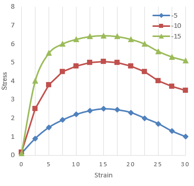
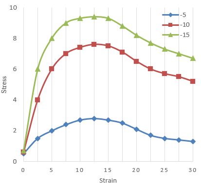
Formula (5) shows that, as a volume latent heat, the K value depends on the difference between the total water content and the unfrozen water content of frozen soil. To acquire the compressive and bending strengths of permafrost, an unconfined test of frozen soil roadbed was carried out at -5℃, -10℃, and -15℃, using frozen soil samples from permafrost road sections.
Figure 1 shows the stress-strain curves of frozen soil samples, and Table 2 records the results of bending strength test on roadbed. The test results indicate that the content of unfrozen water in frozen soil and the strength of cemented ice are greatly affected by temperature. With the decrease of temperature, compressive and bending strengths of frozen soil were greatly enhanced, while the plasticity of the soil plunged. Hence, three properties of frozen soil increased at the same time: strength, temperature dependence, and proneness to brittle failure.
(a) Road section 1
(b) Road section 2
Figure 1. Stress-strain curves of frozen soil samples
Table 2. Results of bending strength test on roadbed
|
Fill type |
Mean ρTJ |
Mean λ |
TC |
Sample size |
Mean compressive strength |
Mean bending strength |
|
A1 |
1,135 |
26.59 |
-6 |
50.6×50.1×90.1 |
1.28 |
1.32 |
|
1,469 |
25.14 |
-12 |
50.2×50.3×92.7 |
5.76 |
2.72 |
|
|
1,671 |
23.25 |
-18 |
50.5×50.7×90.8 |
7.36 |
3.64 |
|
|
A2 |
1,836 |
9.65 |
-6 |
52.3×50.1×90.8 |
2.59 |
1.08 |
|
1,649 |
11.57 |
-12 |
50.2×50.3×91.3 |
7.61 |
1.98 |
|
|
1,427 |
10.36 |
-18 |
48.9×50.6×90.6 |
9.23 |
2.37 |
Table 3. Influence of ice content in soil on the thermal stability of roadbed
|
Level |
1 |
2 |
3 |
4 |
5 |
|
Thaw settlement |
None |
Weak |
General |
Strong |
Extra strong |
|
Freeze heave |
None |
Weak |
General |
Strong |
|
|
Ice content |
A few |
Slightly many |
Strongly many |
Extremely many |
|
2.2 Analysis of factors affecting thermal stability
2.2.1 Engineering geological factors
The upper limit of permafrost is an important factor affecting the thermal stability of roadbed, because the vertical distance between it and the active layer of roadbed directly bears on the ability of frozen soil to resist external thermal disturbances. Let h and γYS be the thaw deformation and compression coefficient of frozen soil, respectively; rDT and rRH be the void ratios of frozen soil in frozen and melt states, respectively; sDT and sRH be the soil layer thicknesses of frozen soil in frozen and melt states, respectively; ∆ζ be the increment in active layer stress. When the active layer of the roadbed undergoes a phase change from frozen state to melt state, the relationship of h with h, sDT and sRH can be expressed as:
$h=\frac{s_{D T}\left(r_{D T}-r_{R H}\right)+\gamma_{Y S} S_{R H} \Delta \zeta}{1+r_{D T}}$ (6)
Formula (6) shows that the thickness of the roadbed active layer increases with its vertical distance to the upper limit position of the permafrost. If the active layer undergoes a phase change from frozen state to melt state, the h value will be relatively large, undermining the thermal stability of roadbed.
In permafrost regions, when the ice content of roadbed soil increases, the roadbed will be more likely to suffer from diseases. Table 3 above presents the influence of ice content in soil on the thermal stability of roadbed. The impact of ice content on roadbed stability is mainly reflected in three aspects: the impact on the mechanical properties of frozen soil, the impact on the ground temperature environment, and the impact on water migration.
The main reason for the thaw settlement of frozen soil roadbed lies in the water damage caused by the excessive water content. For permafrost, the phase change from frozen state to melt state is already in a dynamic equilibrium. The total water content of roadbed is weakly correlated with the frost heave rate of the roadbed, but strongly correlated with the ice content and thaw settlement properties of the roadbed. Let kl be the correlation coefficient; λ0 be the water content at initial thaw settlement. Then, the relationship between the thaw settlement coefficient Φ of frozen soil at levels 1-5 of thaw settlement and total water content λ can be expressed as:
$\Phi=l\left(\lambda-\lambda_{0}\right)$ (7)
where, Φ and λ are linearly and positively correlated with each other. If λ is greater than λ0, Φ will increase with λ, and the frozen soil roadbed will suffer from greater thaw settlement.
2.2.2 Roadbed structural factors
To stabilize frozen soil roadbed and control the probability of roadbed diseases, it is necessary to limit the critical height of the roadbed. Let ∆g be the operating time of the highway; TC be the reasonable height calculated for roadbed; N be the correction coefficient of the frozen soil type; μWD and H be the thermal conductivity coefficient and compressive settlement of the subgrade fill in melt state, respectively. Then, the design critical height TH for a new roadbed can be calculated by:
$T_{H}=0.52 N \mu_{W D} T_{C}+H$ (8)
where, TC can be calculated by:
$T_{C}=0.05 \Delta g-0.02 b+42.86$ (9)
In addition, route direction, pavement type, and foundation treatment also greatly affect the thermal stability of permafrost roadbed. Table 4 shows the impact of road direction on the incidence of roadbed diseases. On the north-south highway, the temperature of the roadbed is basically symmetrically distributed along the centerline, and the aspect factor has a negligeable impact. For highways in other directions, the aspect impact must be considered.
Asphalt pavement has a strong heat absorption effect. If it serves as the roadbed, the annual heat absorption will be much greater than the annual heat output. By contrast, cement pavement is relatively weak in heat absorption, sensitive to roadbed deformation, and high in strength.
Considering the thermal effect of the roadbed, compressive and bending strengths, and the feasibility of roadbed maintenance, materials with high heat reflectivity and small thermal conductivity should be selected in the design phase for the surface layer and structural layer of roadbed, in order to further enhance the thermal stability of the roadbed and effectively reduce the heat transferred from the pavement to the roadbed.
Table 4. Influence of highway direction on the incidence of roadbed diseases
|
Name of highway |
Route length |
Highway direction |
Aspect |
Disease incidence |
|
NT |
354 |
North-south |
East |
2.31 |
|
West |
3.26 |
|||
|
RN |
136 |
West-east |
South |
4.49 |
|
North |
3.47 |
2.2.3 Natural environmental factors
Solar radiation is the main method of heat exchange between the edge of the roadbed and the surrounding air. The amount of solar radiation has a major impact on the temperature changes of the road pavement and the shallow soil of the roadbed. Let C be the heat inflow to the ground; CD and CGD be the direct solar radiation and scattered radiation, respectively; βFS be the reflectivity of the ground; CFN be the effective radiation of the ground. By the physical principles of frozen soil, the roadbed radiation-heat balance in the current year can be described by:
$C=\left(C_{D}+C_{G D}\right)\left(1-\beta_{F S}\right)-C_{F N}$ (10)
The dynamic change of frozen soil hinges on the radiation-heat balance structure in formula (10). In summer, CFN is much smaller than the absorbed radiation (CD+CFN)(1-βFS), and C is positive. In winter, CFN is greater than (CD+CFN)(1-βFS), and C is negative, owing to the limited solar radiation and the reflection of ice and snow on sunlight.
Let CS and CW be the heat inflows to the ground in the summer half year and winter half year, respectively. Then, the thermal stability of the frozen soil roadbed mainly depends on the relationship between CS and CW: If CS≤CW, the mean temperature of frozen soil is not easy to change in the current year, and the roadbed has a high thermal stability; If CS>CW, the mean temperature of frozen soil will increase in the current year, and the strength of frozen soil will degenerate.
Air temperature also affects the stability of frozen soil roadbed during freezing and thawing. The seasonal variation in air temperature brings changes to the temperature of frozen soil, which in turn alters the upper limit position, ice content and active layer thickness.
The stability of frozen soil roadbed is also influenced by rain and snow. The former mainly adjusts temperature, while the latter is a mixed blessing: on the upside, snow protects the roadbed by hindering its heat exchange with the outside; on the downside, snow increases the water content in the roadbed when it melts.
In addition, the wind strength and frequency in permafrost regions directly affect the heat exchange between the edge of the roadbed and the outside, and the evaporation of water.
3.1 Determination of antifreeze mechanism and related parameters
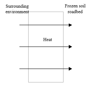
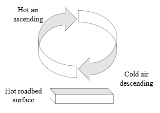
(a) Heat conduction
(b) Heat convection
Figure 2. Heat conduction and convection of frozen soil roadbed
Figure 2 illustrates heat conduction and heat convection of frozen soil roadbed. It can be seen that placing a low thermal conductivity insulation material can effectively prevent external heat from entering the lower soil layer of the frozen soil roadbed. This anti-freeze measure is good at alleviating frost heave and the ensuing uneven deformation of the roadbed. It is highly practical and suitable for permafrost regions and seasonal frozen regions.
Currently, the common industrial thermal insulation materials include polystyrene foam board, new extruded polystyrene board, and polyurethane. The greater the thickness of the thermal insulation layer, the better the anti-freeze effect. Let η be the thickness of the thermal insulation layer; ∆s be the target decrement of freezing depth; μ0 and μ1 be the thermal conductivity coefficients of the roadbed soil and the thermal insulation layer, respectively; L be the correction coefficient. Then, the η value can be calculated by:
$\eta=\frac{L \cdot \Delta s}{\sqrt{\frac{\mu_{0}}{\mu_{1}}-1}}$ (11)
To evaluate the thermal conductivity and model the temperature field of roadbed material, it is critical to capture its parameters like unfrozen water content and freezing temperature. At present, the content of unfrozen water in frozen soil is mostly measured by two methods: the calorimetric method that measures the thermal energy absorbed by ice crystals in frozen soil as they melt, and the temperature measurement by nuclear magnetic resonance (NMR) analyzer, which measures the free induction attenuation of hydrogen nuclei in the magnetic field.
Let q0 be the initial water content of the sample; qWD be the unfrozen water content; B be the signal intensity measured at negative temperature δ; B1 be the signal intensity measured at positive temperature δ; α1 and α2 be empirical coefficients. Then, qWD value can be calculated by:
$q_{W D}=\frac{q_{0} B}{B_{1}}, B_{1}=\alpha_{1}+\alpha_{2} \delta$ (12)
Formula (12) shows that qWD depends on the ratio of measured signal intensity to calculated signal intensity. Let NT be the absolute value of negative temperature. Then, the dynamic equilibrium relationship between qWD and negative temperature can be given by:
$q_{W D}=\alpha_{1} N T^{-\alpha_{2}}$ (13)
The double logarithmic curve of formula (13) is a straight line. Taking q0 of the frozen soil sample as the abscissa of the starting point, and the initial freezing temperature gDT as the ordinate:
$\alpha_{1}=q_{0} g_{D T}^{\alpha_{2}}, \alpha_{2}=\frac{\ln q_{0}-\ln q_{W D}}{\ln N T-\ln g_{D T}}$ (14)
If q0 and gDT are both known, it is only necessary to determine the parameter α2 based on the initial freezing temperatures under two different initial water contents. In this paper, thermocouple and digital voltmeter are used to capture the gDT value of the frozen soil sample. Let gDT be the initial freezing temperature; E be the thermocouple signal recorded by the digital voltmeter; U be the thermocouple calibration coefficient. Then, gDT can be calculated by:
$g_{D T}=E \cdot U$ (15)
3.2 Principle of solving roadbed temperature field
Figure 3. Freezing curve of frozen soil
Figure 3 shows the freezing curve of frozen soil. It can be inferred that, with the elapse of time, the frozen soil temperature gradually decreased. The decrease could be divided into three phases: dropping below zero, sudden rise and stabilization, and falling again. Thus, the temperature of the frozen soil roadbed changes with time. The temperature field of roadbed needs to be investigated by two methods: steady-state thermal analysis and transient thermal analysis.
During the engineering process, the frozen soil roadbed is in a thermally stable state, that is, the sum of the heat passing through a certain section of roadbed in any unit time period is zero. In other words, the energy released by the frozen soil roadbed remains equal to the sum of the energy absorbed from the surrounding environment or sunlight and the energy generated by the internal phase change.
Let [HT] be the heat transfer matrix of different elements determined by the thermal parameters like μ and βDW; {TC} and {HF} be the temperature eigenvector and heat flow rate vector at each test point in the frozen soil roadbed, respectively. Then, the energy balance equation of steady-state thermal analysis can be expressed by:
$[H T]\{T C\}=\{H F\}$ (16)
The load, temperature, and convection of the frozen soil roadbed change dynamically under the transient heat conduction state. Let [HC] be the specific heat capacity matrix, and {TC’} be the derivative of temperature with respect to time, under the transient heat conduction state, respectively. Then, the energy balance equation of transient state thermal analysis can be expressed by:
$[H C]\left\{T C^{\prime}\right\}+[H T]\{T C\}=\{H F\}$ (17)
Let τ be the duration of the entire process. Then, the above parameters can all be written in the form of [HC(τ)], [HT(τ)], and {HF(τ)}. The time-varying state of each parameter can be obtained by substituting the corresponding parameter into the right formula.
During engineering, the structure of the frozen soil roadbed can be likened to a two-dimensional (2D) strip. Hence, the model of frozen soil roadbed can be simply treated as a plane problem. Let TC be the transient temperature of the roadbed soil; DS be the specific heat capacity of the soil at constant pressure; HSIS be the internal heat source intensity of the soil; a and b be the rectangular coordinates; SPRH be the solid phase ratio. After the thermal correction of the phase change from frozen state to melt state, the governing equation for the non-steady state energy transfer on the plane can be updated as:
$\begin{array}{l}
\rho_{T J} D_{S} \frac{\partial T C}{\partial \tau}=\frac{\partial}{\partial a}\left(\mu \frac{\partial T C}{\partial a}\right) \\
+\frac{\partial}{\partial b}\left(\mu \frac{\partial T C}{\partial b}\right)+H S I_{S}+\rho_{T J} K \frac{\partial S P_{R H}}{\partial \tau}
\end{array}$ (18)
This paper aims to construct the basic equation of finite-element calculation for the temperature field of frozen soil roadbed during the phase change from frozen state to melt state. The finite-element transform can be described as:
$\begin{array}{l}
F[T C(a, b, \tau)]=\mu\left(\frac{\partial^{2} T C}{\partial a^{2}}+\frac{\partial^{2} T C}{\partial a^{2}}\right)+H S I_{S} \\
+\rho_{T J} L H \frac{\partial S P_{R H}}{\partial \tau}-\rho_{T J} D_{S} \frac{\partial T C}{\partial \tau}=0
\end{array}$ (19)
The above formula is completed by the Galerkin method of the weighted residual method. To simplify the solution to the partial differential equation of the temperature field, this paper also introduces the weighted residual method and the functional analysis method to process the equation. Let TC1, TC2 ,…,TCm be the undetermined coefficients. The formula of weighted residual method can be defined as:
$\int_{\Re} \omega_{k} F[T C(a, b, \tau)] d a=0$ (20)
where, TC(a, b, τ) can be written in the form of an undetermined coefficient:
$T C(a, b, \tau)=T C\left(a, b, \tau, T C_{1}, T C_{2}, \ldots, T C_{m}\right)$ (21)
Let Γ be the domain of definition, and ωk be the weighting function of the plane temperature field, respectively. Combining formulas (21) and (19):
$\iint_{\Gamma} \omega_{k}\left[\begin{array}{l}
\mu_{S}\left(\frac{\partial^{2} T C}{\partial a^{2}}+\frac{\partial^{2} T C}{\partial a^{2}}\right)+H S I_{S} \\
+\rho_{S} L H \frac{\partial S P_{R H}}{\partial \tau}-\rho_{S} D_{S} \frac{\partial T C}{\partial \tau}
\end{array}\right] d a d b=0$ (22)
where, ωk can be defined as:
$\omega_{k}=\frac{\partial T C}{\partial T C_{j}}$ (23)
The two continuous functions on the domain Γ and the boundary σ are defined as A(a,b) and B(a,b), respectively. Then, the Green’s formula (24) is introduced to correlate the surface integration in Γ with the linear integral on σ. In this way, the boundary condition of function TC(a, b, τ) can be obtained as:
$\iint_{\Gamma}\left(\frac{\partial b}{\partial a}-\frac{\partial A}{\partial b}\right) d a d b=\oint_{\sigma}(A d a+B d b)$ (24)
Combining the transformed form of formula (22) with formula (24), the basic equation for the finite-element calculation of the plane temperature field of the frozen soil roadbed in the phase change from frozen state to melt state can be established as:
$\begin{array}{l}
\frac{\partial O^{\Gamma}}{\partial T C_{j}} \iint_{\Gamma}\left[\begin{array}{l}
\mu_{S}\left(\frac{\partial \omega_{k}}{\partial a} \cdot \frac{\partial T C}{\partial a}+\frac{\partial \omega_{k}}{\partial b} \cdot \frac{\partial T C}{\partial b}\right)- \\
H S I_{S} \omega_{k}-\rho_{S} L H \omega_{k} \frac{\partial S P_{R H}}{\partial \tau} \\
+\rho_{S} \omega_{k} D_{S} \frac{\partial T C}{\partial \tau}
\end{array}\right] \\
d a d b-\oint_{\sigma} \mu_{S} \omega_{k} \frac{\partial G}{\partial m} d h=0
\end{array}$ (25)
Let ε be the boundary condition of the frozen soil roadbed; TC0 and TC(a, b, σ, τ) be the fixed temperature and the corresponding temperature expression, respectively. Then, the first type of boundary condition for frozen soil roadbed with the boundary condition of TC0 or TC(a, b, σ, τ) can be established as:
$\left.T C\right|_{\varepsilon}=T C_{0},\left.T C\right|_{\varepsilon}=T C(a, b, \sigma, \tau)$ (26)
Let HF and HF(a, b, σ, τ) be the fixed heat flux density on the boundary of a frozen soil roadbed and its expression, respectively. Then, the second type of boundary condition for frozen soil roadbed with the boundary condition of HF or HF(a, b, σ, τ) can be established as:
$\begin{array}{l}
-\left.\mu_{S} \frac{\partial T C}{\partial m}\right|_{\varepsilon}=H F,--\left.\mu_{S} \frac{\partial T C}{\partial m}\right|_{\varepsilon} \\
=H F(a, b, \sigma, \tau)
\end{array}$ (27)
Let TCSP and υ be the temperature of a heat transfer roadbed filler and its heat transfer coefficient with frozen soil, respectively. Then, the third type of boundary condition for frozen soil roadbed with the boundary condition of TCSP and υ can be established as:
$-\left.\mu_{S} \frac{\partial T C}{\partial m}\right|_{\varepsilon}=\left.v\left(T C-T C_{S P}\right)\right|_{\varepsilon}$ (28)
To verify the effectiveness of our method in analyzing the thermal stability and temperature field of frozen soil roadbed, the authors tested the temperature field of the road bed, as well as vertical and lateral displacements on multiple layers. The vertical and lateral layered displacement tests consider the vertical displacement of several key nodes on the cross-section, and their lateral displacements at road shoulder and slope toe. Figure 4 shows the displacement field and measurement points of the frozen soil roadbed. The temperature measuring points were arranged at an interval of 0.4m at the centerline, road shoulder, and slope toe on the fill layer, active layer, and upper limit of frozen soil layer, respectively; the measuring points for vertical displacement were deployed at the centerline and shoulder of roadbed, and those for lateral displacement at the shoulder and slope toe.
Figure 4. Displacement field and measurement points of the frozen soil roadbed
The surface humidity changes relatively significantly at the shoulder and slope toe of the frozen soil roadbed, exerting a major impact on the roadbed temperature. Meanwhile, the boundary condition at the centerline on the top surface varies slightly, with a limited impact on ground temperature. This paper chooses the test the centerline temperature on the roadbed cross-section of different test road sections.
(a) Road section 1
(a) Road section 2
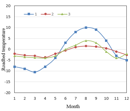
Figure 5. Measured roadbed temperature at centerline in the current year
Figure 5 presents the roadbed temperature measured on the fill layer 1, active layer 2, and upper limit of frozen soil layer 3 in the current year. Obviously, different soil layers exhibited the same change law of temperature. Under the effect of external temperature or sunlight, the fill layer had the largest temperature change range. In the other two layers, the temperature remained relatively stable, due to the deep depth.
(a) Road section 1
(b) Road section 2
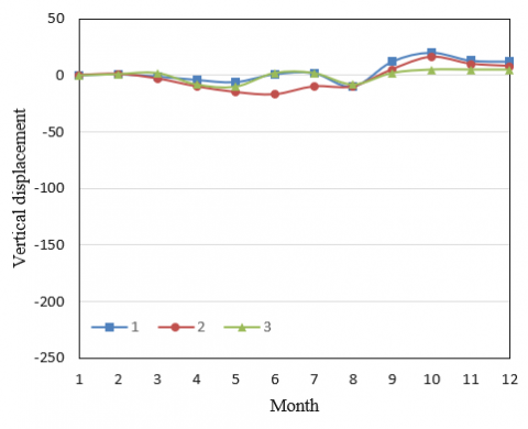
Figure 6. Measured vertical displacement at centerline in the current year
In the current year, the measured roadbed temperature curves at centerline can be divided into several obvious stages: Before April, the roadbed was continuously frozen, and its temperature gradually decreased in the negative range; Starting from May, the roadbed changed from frozen state to melt sate, and its temperature gradually increased; After October, the roadbed was frozen again, and its temperature dropped below zero once more.
The large difference between the curves of different cross-sections comes from the regional difference in ice content and frozen soil layer depth. The same was observed in Figures 6 and 7.
Figure 6 shows the measured vertical displacement at centerline in the current year. Similar to the curves in Figure 5, the vertical displacement curves can be divided into several clear stages: Before April, the roadbed was continuously frozen, some soil layers with low groundwater level experienced frost heave, and the vertical displacement tended to develop upward; After May, the roadbed changed from frozen state to melt sate, the temperature rose back to above zero, and the vertical displacement developed quickly, but at an increasingly slow rate. The different soil layers had similar temperature change law, and basically the same trend of cumulative vertical displacement.
(a) Road section 1
(b) Road section 2
Figure 7. Measured lateral displacement at centerline in the current year
Figure 7 shows the measured lateral displacement at centerline in the current year. When the roadbed temperature field was in the negative state with falling temperature, the fill layer had a large lateral displacement. When the roadbed temperature field was in the positive state with rising temperature, the phase change water could only be discharged along the side of the roadbed, because the roadbed was frozen; In this case, an inflection point was formed on the curve, indicating the directional change of lateral displacement. When the roadbed temperature field rose to above zero, the lateral displacement of each soil layer increased at a growing speed.
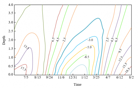
Figures 8 and 9 present how the roadbed temperatures at centerline and slope top change with depth in the current year, respectively. It can be seen that the maximum freezing depths at the center and on the slope of the frozen soil roadbed was 1.2m and 1.7m, respectively.
Because the frost heave and thaw settlement of the roadbed vary from position to position. The freezing and thawing time of the roadbed soil at the center and on the slope could be derived from the two figures. It can be seen that different measuring points captured different frosting and thawing time. If the freezing time is long and thawing time is short, then the freezing of frozen soil is unidirectional, while the thawing is bidirectional. In addition, Figures 8 and 9 display the same change law of temperature as indicated by the previous analysis.
Figure 8. Variation of centerline temperature with depth in the current year
Figure 9. Variation of slope tope temperature with depth in the current year
This paper probes deep into the distribution law of temperature field and thermal stability of roadbed in permafrost regions. Firstly, three types of factors affecting thermal stability were analyzed, including engineering geological factors, roadbed structural factors, and natural environmental factors. Then, the antifreeze mechanism of frozen soil roadbed was expounded, and the temperature field of the roadbed with low thermal conductivity insulation material was analyzed by two methods, namely, steady-state thermal analysis and transient thermal analysis. Afterwards, the authors detailed the solving process of roadbed temperature field. Finally, our method was proved effective in analyzing thermal stability and temperature field of frozen soil roadbed, through temperature field test, and layered tests on vertical and lateral displacements.
This work was supported by National Natural Science Foundation of China (Grant No.: 51378164); Natural Science Foundation of Heilongjiang (Grant No.: E2016045).
[1] Liu, Z.Q., Ma, W., Zhou, G.Q., Niu, F.J., Duan, Q.J., Wang, J.Z., Zhao, G.S. (2005). Simulated experiment study on the temperature field of frozen subgrade modulated by horizontal pipes. Chinese Journal of Rock Mechanics and Engineering, 24(11): 1827-1831.
[2] Stoyanovich, G.M., Pupatenko, V.V., Maleev, D.Y., Zmeev, K.V. (2017). Solution of the problem of providing railway track stability in joint sections between railroad facilities and subgrade. Procedia Engineering, 189: 587-592. https://doi.org/10.1016/j.proeng.2017.05.093
[3] Chitragar, S.F., Shivayogimath, C.B., Mulangi, R.H. (2020). Study on strength and volume change behavior of stabilized black cotton soil with different pH of soil-lime mixes for pavement subgrade. International Journal of Pavement Research and Technology, 14: 543-548. https://doi.org/10.1007/s42947-020-0117-x
[4] Kang, Q., Wang, X.M., Pu, H., Wang, S. (2016). Analysis of subgrade stability in karst area based on variable weight theory-uncertainty measurement method. Journal of Northeastern University (Natural Science), 37(3): 435. https://doi.org/10.12068/j.issn.1005-3026.2016.03.028
[5] Adeyanju, E., Okeke, C.A., Akinwumi, I., Busari, A. (2020). Subgrade stabilization using rice husk ash-based geopolymer (GRHA) and cement kiln dust (CKD). Case Studies in Construction Materials, 13: e00388. https://doi.org/10.1016/j.cscm.2020.e00388
[6] Neupane, M., Han, J., Parsons, R.L. (2020). Experimental and analytical evaluations of mechanically-stabilized layers with geogrid over weak subgrade under static loading. In Geo-Congress 2020: Engineering, Monitoring, and Management of Geotechnical Infrastructure, 597-606. https://doi.org/10.1061/9780784482797.058
[7] Walkenbach, T.N., Han, J., Parsons, R.L., Li, Z. (2020). Effect of geogrid stabilization on performance of granular base course over weak subgrade. In Geo-Congress 2020: Geotechnical Earthquake Engineering and Special Topics, 527-535. https://doi.org/10.1061/9780784482810.055
[8] Behnood, A., Olek, J. (2020). Full-scale laboratory evaluation of the effectiveness of subgrade soil stabilization practices for Portland cement concrete pavements patching applications. Transportation Research Record, 2674(5): 465-474. https://doi.org/10.1177/0361198120916476
[9] Akpinar, M.V., Pancar, E.B., Şengül, E., Aslan, H. (2018). Pavement subgrade stabilization with lime and cellular confinement system. The Baltic Journal of Road and Bridge Engineering, 13(2): 87-93.
[10] Chibuzor, O.K., Van Duc, B. (2018). Predicting subgrade stiffness of nanostructured palm bunch ash stabilized lateritic soil for transport geotechnics purposes. Journal of GeoEngineering, 13(1): 3. https://doi.org/10.6310/jog.2018.13(1).3
[11] Liu, Z.Q., Ma, W., Zhou, G.Q., Niu, F.J., Wang, J.Z., Chang, L.W., Zhou, J.S. (2005). Simulating experiment for temperature field of frozen subgrade using regulation-tubes. Journal of China University of Mining and Technology, 15(1): 21-25.
[12] Song, H., Xie, Z.S., Zheng, H.Y., Zhang, W. (2007). Numerical simulation for temperature field of subgrade on seasonal frozen area. In International Conference on Transportation Engineering, 1753-1758. https://doi.org/10.1061/40932(246)287
[13] Tan, Y.Q., Xu, H.N., Zhou, C.X., Zhang, K., Chen, F.C. (2011). Temperature distribution characteristic of subgrade in seasonally frozen regions. Harbin Gongye Daxue Xuebao (Journal of Harbin Institute of Technology), 43(8): 98-102.
[14] Al-Jhayyish, A.K., Sargand, S.M. (2017). Incorporating the strength provided by subgrade stabilization in the flexible pavement design procedures. Geotechnical Testing Journal, 41(1): 117-131. https://doi.org/10.1520/GTJ20160317
[15] Buslov, A., Margolin, V. (2017). The interaction of piles in double-row pile retaining walls in the stabilization of the subgrade. In Energy Management of Municipal Transportation Facilities and Transport, 769-775. https://doi.org/10.1007/978-3-319-70987-1_81
[16] Murthy, G.V., Krishna, A.V., Rao, V.V.P. (2017). An experimental study on partial replacement of clayey soil with an industrial effluent: Stabilization of soil subgrade. In International Congress and Exhibition Sustainable Civil Infrastructures: Innovative Infrastructure Geotechnology, pp. 337-348. https://doi.org/10.1007/978-3-319-61902-6_26
[17] Chang, L.W., Xu, Y.J., Yue, J.C. (2011). Simulation experiment of dynamic responses of high temperature frozen subgrade to dynamic loading. Journal of the China Railway Society, 33(11): 80-84.
[18] Tai, B., Yue, Z., Sun, T., Qi, S., Li, L., Yang, Z. (2021). Novel anti-frost subgrade bed structures a high speed railways in deep seasonally frozen ground regions: Experimental and numerical studies. Construction and Building Materials, 269: 121266. https://doi.org/10.1016/j.conbuildmat.2020.121266
[19] Tregubov, O.D. (2015). Experience in using GPR to study new frozen-ground formations in subgrade structures. Soil Mechanics and Foundation Engineering, 52(5): 286-291. https://doi.org/10.1007/s11204-015-9343-7
[20] Akimov, S., Kosenko, S., Bogdanovich, S. (2019). Stability of the supporting subgrade on the tracks with heavy train movement. In International Scientific Siberian Transport Forum, 1116: 228-236. https://doi.org/10.1007/978-3-030-37919-3_22
[21] Kovalchuk, V., Sysyn, M., Nabochenko, O., Pentsak, A., Voznyak, O., Kinter, S. (2019). Stability of the railway subgrade under condition of its elements damage and severe environment. In MATEC Web of Conferences, 294: 03017.
[22] Wysocki, G., Ksi, B., Kucz, M. (2017). The influence of a low bearing subgrade on the stability of a shared street (woonerf) foundation. Procedia Engineering, 172: 1252-1260. https://doi.org/10.1016/j.proeng.2017.02.147
[23] Aswathy, C.M., Raj, A.S., Sayida, M.K. (2021). Effect of bio-enzyme—chemical stabilizer mixture on improving the subgrade properties. In Problematic Soils and Geoenvironmental Concerns, 88: 779-787. https://doi.org/10.1007/978-981-15-6237-2_63
[24] Komaravolu, V.P., GuhaRay, A., Tulluri, S.K. (2020). Subgrade stabilization using alkali activated binder treated jute geotextile. In Problematic Soils and Geoenvironmental Concerns, 88: 343-354. https://doi.org/10.1007/978-981-15-6237-2_29
[25] Kumar, V., Panwar, R.S. (2019). Mitigation of greenhouse gas emissions by fly ash stabilization and sisal fibre reinforcement of clay subgrade for road construction. In IOP Conference Series: Earth and Environmental Science, 219(1): 012020. https://doi.org/10.1088/1755-1315/219/1/012020
[26] Apriyanti, Y., Fahriani, F., Fauzan, H. (2019). Use of gypsum waste and tin tailings as stabilization materials for clay to improve quality of subgrade. In IOP Conference Series: Earth and Environmental Science, 353(1): 01204. https://doi.org/10.1088/1755-1315/353/1/012042
[27] Ikeagwuani, C.C., Nwonu, D.C. (2019). Resilient modulus of lime-bamboo ash stabilized subgrade soil with different compactive energy. Geotechnical and Geological Engineering, 37(4): 3557-3565. https://doi.org/10.1007/s10706-019-00849-6
[28] Mishra, S., Sachdeva, S.N., Manocha, R. (2019). Subgrade soil stabilization using stone dust and coarse aggregate: A cost effective approach. International Journal of Geosynthetics and Ground Engineering, 5(3): 1-11. https://doi.org/10.1007/s40891-019-0171-0
[29] Tavakol, M., Hossain, M., Tucker-Kulesza, S.E. (2019). Subgrade soil stabilization using low-quality recycled concrete aggregate. In Geo-Congress 2019: Geotechnical Materials, Modeling, and Testing, pp. 235-244. https://doi.org/10.1061/9780784482124.025
[30] Ikeagwuani, C.C., Obeta, I.N., Agunwamba, J.C. (2019). Stabilization of black cotton soil subgrade using sawdust ash and lime. Soils and Foundations, 59(1): 162-175. https://doi.org/10.1016/j.sandf.2018.10.004