Brihmat Mostefa* | Refassi Kaddour | Douroum Embarek | Kouadri Amar
© 2021 IIETA. This article is published by IIETA and is licensed under the CC BY 4.0 license (http://creativecommons.org/licenses/by/4.0/).
OPEN ACCESS
Centrifugal compressors have been used in many areas of the machinery. The centrifugal compressor design is very complex, and a unique design system needs to be developed. A centrifugal compressor design system should be easy to use in interface and also flexible for inputs and outputs. The design tool also needs to be able to predicate the compressor performance in a fairly accurate level. In this study, we have developed a general analyses and optimization approach in the design and performance analysis of centrifugal turbomachines. This approach is based on different methods starting from a 1D approach up to the 3D study of the internal flow. It presents itself as a robust procedure for predicting and understanding the phenomena associated with the operation of turbomachines, but also for predicting performance. Current design system includes initial parameter studies, throughflow calculation, impeller design. The main improvements of the design system are adding the interface to allow users easy to use, adding the input and output capabilities and modifying few correlations. Current design system can predict the blade loading and compressor performance better compared with original design system. To check the aerodynamic appearance of the centrifugal compressor impeller blades, we must change the impeller dimensions and focus on changing axial length, but when changing the blade numbers, the model that improved efficiency and power at the same time introduced a design with a 0.274% and 10.735% improvement in each respectively in comparison to the initial impeller at the design point.
turbomachinery designs, impeller, thermodynamics, aerodynamics, centrifugal compressor, CFD
The design of the impeller is very critical for a compressor stage. The proper blade loading distributions with minimums boundary layer distortions can significantly improve the compressor performance. The estimations of the blade loadings are improved in the current studies to closer to CFD results. Many design optimizations and CFD analysis have been used for improving the impeller aerodynamic designs [1-9]. Impeller aerodynamic design not only affects the impeller efficiency but also affects the performance of downstream diffuser and volute. It is important for an impeller to achieve a high-efficiency design with relative uniform exit flow. The design of centrifugal impeller is subject to multidisciplinary and multi-objective optimizations among aerodynamics, structure, and rotor dynamics.
Turbines produce the power by expanding fluids through drop pressure or head, and temperature. Turbines are widely used in aerospace, power generations, automobile, and aerospace, etc. Successful turbomachine designs are very critical. In the concept design stage of the turbomachines, it is very important to have a good estimation of the compressor or turbine performance from choosing preliminary parameters [10, 11].
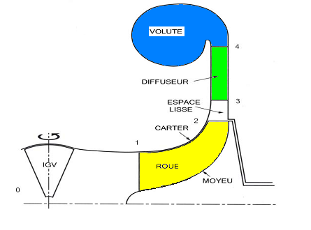
Centrifugal compressors are identified as radial turbomachines. This type of compressor is composed of three main elements, namely, the rotating part or impeller, and stationary parts; diffuser and manifold. An important part up stream of the impeller is the inducer duct.
Air is sucked into the impeller eye and whirled round at high speed by the vanes on the impeller disc. The normal practice is to design the compressor so that about half the pressure rise occurs in the impeller and half in the diffuser [12].
Large variations in pressure contours are not observed when crossing the boundary between the two major components, but noticeable gradients are present at the diffuser outlet because of the sudden increase in width at the volute inlet. Still heavier distortions in the pressure are present at the volute tongue because of the large incidence, creating a separation like flow on the suction side of the tongue [13].
Niazi et al. [14] employed a sector-domain (or passage) between two successive blades) in the impeller for numerical calculations for the flow in an impeller of single-stage centrifugal compressor. He generated a grid of 400,000 nodes; next he increased the number of nodes till 1.8 million nodes in a mesh sensitivity analysis. Code validation with achieved via comparison with experimental data. He was able to simulate surge and studied surge control by air-injection. He also examined other parameters such as velocity and total pressure.
Aghaei et al. [15] studied how a good compressor can be designed and modeled with CFD steady models and to explain reasons for discrepancies between experiment (1D design) and 3D CFD analysis. Design/methodology/approach – A model with only one impeller channel was used to compare 1D design data, which were obtained from centrifugal compressor design code, written and developed by the authors. The numerical results with respect to performance data showed quite good agreement with experimental data at and near the operating point of best efficiency. Originality/value – This paper offers a combined 1D and 3D numerical approach in turbo machinery design, especially in radial compressible turbo machines design.
Xu and Muller [16] presented a detailed flow simulation in the volute of a single-stage centrifugal compressor. Their computationnels domain had 782,000 nodes. The “Frozen-rotor” method is used at interfaces between rotating and stationary elements. They considered a full-domain flow study and plotted the pressure distribution of the volute.
Yutaka et al. [17] carried out a numerical and experimental study of the centrifugal-compressor noise affected by the flow in the tapered diffuser. Experimentally, they presented advanced experimental setup. Numerically, 3D steady model was used to simulate flow. The numerical model utilized a full-domain mesh (single-stage) and a sliding mesh method.
Ling et al. [18] simulated a small centrifugal compressor undertaken at the MPG and KJ66 gas turbine design. They studied improving the efficiency of the compressor by increasing the impeller diameter from 66 mm to 71 mm. They found that the performance of the new design is better than the old one within a certain operating range.
An efficient optimization approach to centrifugal impeller blades is developed and applied to the design of a 3D impeller using; UDM, CFD, regression analysis method, and genetic algorithm. Global optimization of the approximate function is obtained by genetic algorithms. Taking maximum isentropic efficiency as objective function, this optimization approach has been applied to the optimum design of a certain centrifugal compressor blades [19]. The results, compared with those of the original one, show that isentropic efficiency of the optimized impeller has been improved which indicates the effectiveness of the proposed optimization approach such as CFD, structural dynamics, and thermal analysis combined with the emergence of improved optimization algorithms makes it possible to perform blade shape automatic optimization process.
Tang et al. [20] studied numerically a 3D impeller and vaneless diffuser of a small centrifugal compressor. The influence of impeller tip clearance on the flow field of the impeller was investigated. Then, a new partially shrouded impeller was designed. They used a sector-domain and 110,000 grid points. Numerical results show that the secondary flow region becomes smaller at the exit of the impeller. Better performance is achieved in comparison with the un-shrouded impeller.
Centrifugal compressors are used in many heat pumps and refrigeration systems. Radial vaneless diffuser is a principal component in these compressors. Therefore, Shaaban [21] in his article aims at improving the centrifugal compressor performance by optimizing the design of the radial vaneless diffuser. Two radial vaneless diffuser geometries were proposed, investigated and numerically optimized. The optimization aimed at minimizing the diffuser loss coefficient and maximizing the pressure coefficient. Simulations were performed by solving the Reynolds averaged Navier–Stokes equation under 2D axisymmetric condition. To the combination of centrifugal force, aerodynamic pressure and thermal load results in non-uniform tip clearance profile.
Kim et al. [22]. in his article A series of aero-thermo-mechanical analyses were carried out to predict the running tip clearance and the effects of impeller deformation on the performance using two different centrifugal compressors (blade type A and B). In operation, impeller deformation due displacement occurs at the leading edge tip of the impeller blade but maximum stress takes place at the blade root of the impeller.
The design of the impeller is very critical for a compressor stage. The proper blade loading distributions with minimums boundary layer distortions can significantly improve the compressor performance. The estimations of the blade loadings are improved in the current studies to closer to CFD results. Many design optimizations and CFD analysis have been used for improving the impeller aerodynamic designs [23-31]. Impeller aerodynamic design not only affects the impeller efficiency but also affects the performance of downstream diffuser and volute. It is important for an impeller to achieve a high-efficiency design with relative uniform exit flow. The design of centrifugal impeller is subject to multidisciplinary and multi-objective optimizations among aerodynamics, structure, and rotor dynamics.
The objective of the approach presented in this article is study aerodynamic performance. For this, we used an approach based on the reduction of the sources internal to the impeller (it is the object of a selection of the aerodynamic parameters according to the acoustic computations), and using the software ANSYS CFX and the method k - ε. For performance at the nominal point, we applied the criteria suggested by the literature, the main differences between the original impeller and the optimized one being the value of the slowing down. To show the validity of the correlations and models proposed in this study the modifications have the main modified parameters correspond to the impeller: the axial length, the number of blades.
To optimize the impeller of this compressor and reduce turbulence losses, we have changed some parameters of the original turbocharger impeller. But we finally found that when you change the numbers of the blades, you get good results for the performance of the central compressor.
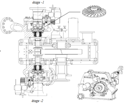
2.1 Description of the centrifugal compressor MAN-Turbo
The turbocharger man -turbo type RG028/02-l2 (Figure 1) consists of a single helical gear wheel and compressor stages. A large gear wheel drives a gear shaft. On the end faces of the pinion shaft are screwed in the axial direction, the moving wheels, with a Hirth lock. The axial forces of the pinion shaft are transmitted to the large gear by thrust collars. The thrust bearing of the shaft of the large gear wheel absorbs the axial force resulting therefrom. The compressor ratio R1S / R2 = 0.53.
Each compressor stage consists of a cantilevered mobile impeller, surrounded by a volute casing. The housings are supported by vertical flanges arranged on the speed adapter. In the housings are housed the blade supports and the input insert.
The movable impelles of stages 1, 2 are in closed construction. Each of these impelles is separated from its volute casing by axial and radial seals. impeller linings are designed as non-contact labyrinth liners. They seal between the inlet and outlet sides of each stage of the compressor. The operating conditions of the centrifugal compressor studied in this specification are presented in Table 1.
Table 1. Compressor operating conditions Man-Turbo
|
Amount |
Specified value |
|
total pressure total temperature flow of mass rotation speed operating fluid polytropic efficiency |
Pt1 = 16 bar Tt 1= 68.4℃ m˙ = 0.28 kg/s N = 21592 tr/min Gaz η=79.39 |
Figure 1. Sectional view of the speed adapter compressor
Figure 2 shows the original impeller is given from experimental executions.
Man-turbo centrifugal compressor, impeller geometry and experimental design data. The main dimensions of the original wheel are summarized in Table 2.
Figure 2. Original impeller geometry
Table 2. Main dimensions of the original impeller
|
Geometric data of the original impeller |
Dimensions |
|
outlet diameter blade height at outlet number of blades metal angle at exit input radius for foot R1h input radius for blade head R1s |
D2 = 275 mm b2 = 10 mm ZPR = 18 βp2 = 60º R1h = 43 mm R1S =73mm |
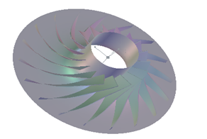
Figure 3 shows a 3D view of the original man-turbo compressor impeller obtained from the ANSYS Workbench software "CFX-BladeGEN".
Figure 3. 3D visualization of the original impeller man turbo CFX-BladeGEN
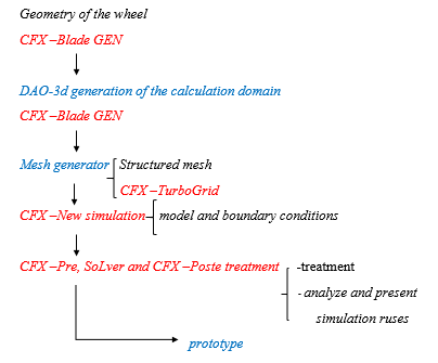
The numerical simulation has proven to be well suited and efficient for accomplishing the task of dimensioning and optimizing a centrifugal wheel. However, the development of computer resources and digital techniques have allowed the emergence of CFD codes capable of analyzing the three-dimensional structure of internal flows. In this work, two objectives will be followed using CFD software. That is to say: their use represents, at the same time, the finest optimization but also the final step of the design process and the validation of the previous steps. Presented CFD codes are commercial software: CFX-BladeGEN, CFX-TurboGrid. Automatic or operator-controlled links allow dialogue between CFX-Pre, CFX-Solver and CFX-Post.
3.1 Governing equations
$\frac{\partial \rho }{\partial t}+\frac{\partial }{\partial {{x}_{i}}}\left( \rho {{V}_{i}} \right)=0$ (1)
$\frac{\partial \left( \rho {{V}_{i}} \right)}{\partial t}+\frac{\partial }{\partial {{x}_{j}}}\left( \rho {{V}_{i}}{{V}_{j}} \right)=-\frac{\partial p}{\partial {{x}_{i}}}+\frac{\partial {{\tau }_{ij}}}{\partial {{x}_{j}}}$ (2)
where, p is the static pressure, and is the viscous stress tensor given by
${{\tau }_{ij}}=\left[ \frac{\partial {{V}_{i}}}{\partial {{x}_{j}}}+\frac{\partial {{V}_{j}}}{\partial {{x}_{i}}}+\frac{2}{3}\frac{\partial {{V}_{l}}}{\partial {{x}_{l}}} \right]$ (3)
$\frac{\partial \left( \rho E \right)}{\partial t}+\frac{\partial }{\partial {{x}_{i}}}\left[ {{V}_{i}}\left( \rho E+p \right) \right]=\frac{\partial }{\partial {{x}_{i}}}\left( K\frac{\partial t}{\partial {{x}_{i}}}-\sum\limits_{j}^{{}}{{{h}_{j}}{{J}_{i}}+\left( {{V}_{i}}{{\tau }_{ij}} \right)} \right)h$ (4)
1-Equation of turbulence energy (k):
$\frac{\partial }{\partial t}\left( \rho k \right)+\frac{\partial }{\partial {{x}_{i}}}\left( \rho k{{u}_{i}} \right)=\frac{\partial }{\partial {{x}_{j}}}\left[ \left( \mu +\frac{{{\mu }_{t}}}{{{\sigma }_{k}}} \right)\frac{\partial k}{\partial {{x}_{j}}} \right]-\rho E$ (5)
2-Equation of rate of dissipation of turbulence kinetic energy (E):
$\frac{\partial }{\partial t}\left( \rho E \right)+\frac{\partial }{\partial {{x}_{i}}}\left( \rho E{{u}_{i}} \right)=\frac{\partial }{\partial {{x}_{j}}}\left[ \left( \mu +\frac{{{\mu }_{t}}}{{{\sigma }_{E}}} \right)\frac{\partial E}{\partial {{x}_{j}}} \right]+{{C}_{1E}}\frac{E}{k}{{C}_{3E}}-{{C}_{2E}}\frac{{{E}^{2}}}{k}$ (6)
The model constants $C_{1 E}, C_{2 E}, C \mu, \sigma k,$ and $\sigma \epsilon$ have the following default values: $C 1 \mathrm{E}=1.44, C 2 \mathrm{E}=1.92, C \mu=0.09$, $\sigma k=1.0$ and $\sigma_{E}=1.3$
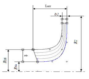
Pre-dimensioning is defined as the step that sets the main characteristic dimensions of the machine at the stations recalled in Figure 4.
Impeller: spokes at the entry for the foot and the blade head: R1h and R1S, exit radius R2 and output blade height: b2. Wedge angles of the blades βp1s, βp1h. Axial length Lax, the value of the angle βp2, is optionally refined during this step. This step relies mainly on two approaches: (I) the use of empirical criteria and (II) the use of 1D-prediction tools.
Figure 4. Schematic view of a centrifugal compressor stage
Radius at the head the pre-dimensioning of the impeller begins with the establishment of the radius at the input casing, under the constraint given for R1h.
Japikse [32] recommend minimizing the number of mach in mind the theoretical justification is to minimize friction losses, related at the speed level.
Note that this is also beneficial for acoustics. For a feed without pre-rotation, the relative velocity of the fluid at the top of the blade is written:
${{W}_{1S}}=\sqrt{{{U}_{1S}}^{2}+{{C}_{1S}}^{2}}$ (7)
Once the overall characteristics of if the radius to the casing is reduced, the peripheral speed of the blade (U1S = R1S. Ω) decreases. However, as the debiting section decreases the retention of the flow rate leads to an increase in C1S. Thus, W1S is influenced by two contradictory effects: An optimum of R1S exists to minimize the number of relative mach inputs.
The optimum must be calculated by assuming the meridional velocity ratio (Rvm = C1s /0.5 (C1h + C1s)). All calculations made this optimum is expressed:
${{R}_{1S}}_{optimum}=\sqrt{{{R}_{1h}}^{2}+2{{\left( \frac{{{R}_{vm}}\dot{m}}{\Omega {{\rho }_{1}}\pi } \right)}^{2/3}}}$ (8)
The value obtained depends strongly on the meridian speed ratio and the radius at the hub. Placing of the blades in the foot and at the head as a first approximation, it is possible to evaluate the relative angle of the inlet flow β1 once R1h and R1S fixed. Assuming the one-dimensional flow, we can show that:
${{\beta }_{1S}}={{\tan }^{-1}}\frac{{{U}_{1S}}}{{{C}_{1S}}}={{\tan }^{-1}}\frac{{{R}_{1S\omega }}}{\dot{m}/{{\rho }_{1}}\pi \left( {{R}^{2}}_{1S}-{{R}^{2}}_{1h} \right)}$ (9)
For the flow at the head, the choice of blade pitch can then be initiated by using a criterion for the incidence I (defined as the difference between the relative angle of the incident flow and the pitch of the blade). Number of blades of the impeller resulting from an optimization between friction and sliding is given by the relation:
ZPR = 25*cos (β2)/nsq (10)
The axial length Lax is a parameter that significantly influences the aerodynamic performance, but also: (I) the size of the stage, (II) the dynamics of the shaft, (III) the mechanical stresses in the impeller. From the point of view of aerodynamics.
Figure 5. Scheme for conducting impeller analysis by CFD
The axial length is given by the following relationship:
$\frac{{{L}_{ax}}}{{{R}_{2}}}=2\sqrt{K\left( {{M}^{*}}_{1S}+{{K}_{2}} \right)\left( 1-\frac{{{R}_{1S}}-{{R}_{1h}}}{2{{R}_{2}}} \right)\frac{{{R}_{1S}}-{{R}_{1h}}}{{{R}_{2}}}}$ (11)
where, K1 = 0.28 and K2 = 0.8. Thus, for typical values of R1h, R1S and R2, the ratio Lax / R2 varies between 0.62 and 0.77 when the number of mach varies between 0.6 and 0.9. The number of mach of the input and the exit of the impeller.
${{M}^{*}}_{1}=\frac{{{W}_{1}}}{\sqrt{\gamma R{{T}_{1}}}}$; ${{M}^{*}}_{2}=\frac{{{W}_{2}}}{\sqrt{\gamma R{{T}_{2}}}}$ (12)
The objective of this study:
-Check the execution impact due to the change of some geometric parameters.
-Check the execution impact due to the change in the number of blades.
Figure 5 shows the different steps taken during the three-dimensional simulation of the turbo centrifugal compressor impeller.
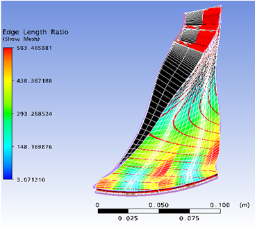
The diversity of mesh generation methods can result in many ways of characterizing a computing grid. We consider here the case of meshes generated with ANSYS Workbench software "TurboGrid". A first choice is the set of topology H / J / C / L-Grid, for the study of turbomachines the axisymmetric flow hypothesis allows the simplification of the single-channel calculation domain interaubages. The different boundaries for modeling a channel of the centrifugal compressor impeller are shown schematically in Figure 6.
Figure 6. Mesh of the original impeller. Blade to blade
Figure 7. Centrifugal impeller; Structured mesh
The second level is a further study for the study of internal flow. It begins with the creation of a structured mesh using the CFX-TurboGrid software (Figure 7).
Table 3 shows some execution parameters.
Table 3. Compressor performance results. Original impeller
|
input power (w) |
407336.0000 |
|
intake flow coefficient |
0.0123 |
|
outlet flow coefficient |
0.0898 |
|
total pressure ratio |
1.9948 |
|
total temperature ratio |
1.2354 |
|
isentropic efficiency |
92.7412 |
|
polytropic efficiency |
93.4136 |
We consider here the case of meshes generated with ANSYS Workbench software "TurboGrid". A first choice is the set of topology H / J / C / L-Grid. The mesh data are as follows:
Table 4. Mesh data. Topology H / J / C / L-Grid
|
Characteristics |
Total nodes |
Total element |
|
mesh |
33143 |
28948 |
Using ANSYS CFX -post software, the most important results for the simulation of the original man turbo geometry have been deduced. Table 4 shows the compilation of some execution parameters.
5.1 Figures produced for the CFX
The CFX is a software that allows quick and easy visualization of simulation results, gives various graphs of various parameters in different plans. In this section they will be shown to the graphs obtained in the simulation of the man-turbo compressor.
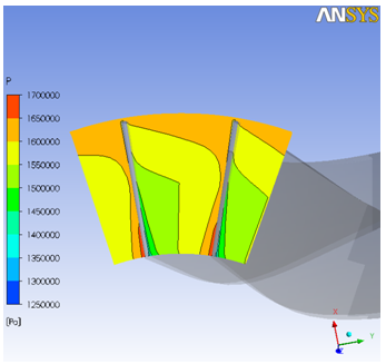
The gas, an irrotational fluid, enters the impeller, tends to create a vortex of the opposite direction of rotation (Figure 8). This takes a region of little pressure on one side of the wheel's blade, known as the suction side; while on the other it is of greater pressure, known as pressure side. This effect at the leading edge and edge of fuit in Figures 9 (a, b). The Z-axis coincides with the axis of the wheel and its direction is in the direction of the entry of the wheel. As in modeling the direction of rotation, it is negative in the Z axis, the edge of the attack means that the rotation goes from right to left. Due to the format of the impeller, the direction of rotation in the edge of the leak is opposite, that is to say, it goes from left to right.
It can be visualized clearly in Figures 9 (a, b) and the side of the blade aspiration, where the value of pressure is less throughout the leading edge and edge of leak, and in the dawn opposition side the value of the pressure is greater in all this region.
A point can be seen in Figure 9 b where the pressure is greater. Possible explanation for this is the formation of the mats in the outlet of the impeller making the fluid to return to the impeller, being created a region of stagnation raising the pressure.
Figure 8. Direction of rotation z
a) Pressure in the leading edge
b) Pressure in the edge of leaks
Figure 9. Pressure in the leading edge and the trailing edge
Table 5. RNG results k -ε original impeller parameter
|
Parameter |
Entrance |
Leading edge |
edge of leaks |
Exit |
|
P static (pa) |
1677490.0000 |
1675170.000 |
2485910.000 |
2593270.000 |
|
P total (pa) |
1688770.0000 |
1673950.000 |
3402740.000 |
3368670.000 |
|
P t (rot) (pa) |
1676890.0000 |
1664860.000 |
1601420.000 |
1596370.000 |
|
T static (K) |
339.9550 |
339.4260 |
386.9860 |
391.9690 |
|
T total (K) |
341.8260 |
341.7370 |
423.8920 |
422.9850 |
|
Tt (rot) (K) |
341.1140 |
341.0750 |
341.1350 |
341.1240 |
|
Enthalpy (J/kg) |
43153.4000 |
43114.3000 |
43174.2000 |
43163.4000 |
|
Entropy (J/kg) |
-670.4250 |
-668.4220 |
-657.1680 |
-656.3220 |
|
Mach abs |
0.1644 |
0.1906 |
0.6838 |
0.6228 |
|
Mach rel |
0.3431 |
0.3320 |
0.1554 |
0.2424 |
|
u (m/s) |
134.5690 |
134.3160 |
310.3630 |
333.5010 |
|
Cm(m/s) |
52.3589 |
57.7330 |
27.8787 |
26.3787 |
|
Cu (m/s) |
-46.7831 |
-73.1338 |
-271.8680 |
-243.0850 |
|
C (m/s) |
84.7199 |
105.7770 |
274.0240 |
244.9330 |
|
Wu (m/s) |
87.7860 |
61.1842 |
38.4967 |
90.4162 |
|
W (m/s) |
103.6210 |
88.5834 |
48.6757 |
95.3097 |
|
Flow Angle: Alpha |
75.5287 |
-60.4172 |
77.4171 |
39.2016 |
|
Flow Angle: Beta |
-75.1775 |
-94.4162 |
-57.0229 |
-74.9403 |
Table 5 shows RNG results k –ε original man turbo wheel parameter.
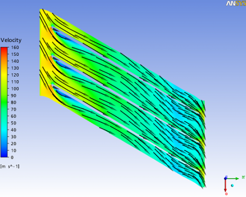
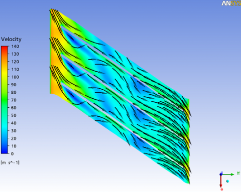
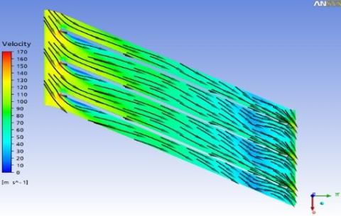
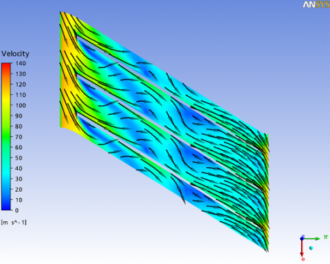
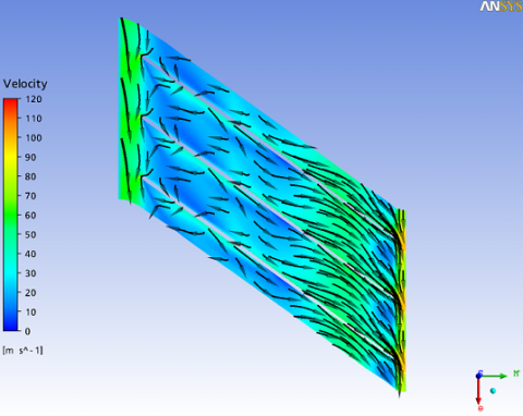
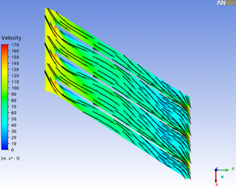
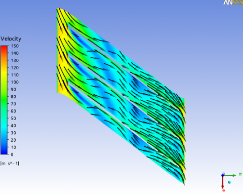
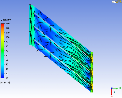
CFX produces vectors of this velocity for 20, 50 and 80% of the normal blade size, shown in Figures 10 to 12. These figures allow to remove some conclusions, namely:
• The speed reaches maximum values in the upper blade part of the impeller, next to the crankcase.
• A stagnation region exists, already detected before the results. The pressure in the region next to the wheel output, in which the speed reaches minimum values. This effect is greater in the upper blade part, near the crankcase.
• As commented in all this work, it is exactly in this region where vortexes and mats occur, leading to the reduction of the gas bill area so that the speed next to the wall is almost zero. It can be clearly visualized the separation mat, explaining the high values of mach in the output of the impeller.
These last three figures clearly explain the angle variation along the edge of the leak.
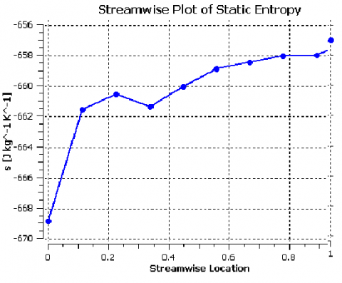
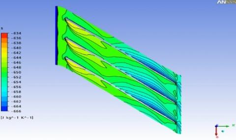
The losses inside the wheel can be visualized by the graphs and curves of the entropy produced by the CFX. Entropy is a thermodynamic property in which it is necessary to make an analysis with respect to a value of the reference to know where its greatest variation occurs. This analysis helps to avoid where the biggest losses occur.
Figure 10. Velocity at span of 20℅, blade to blade
Figure 11. Velocity at span of 50℅, blade to blade
Figure 12. Velocity at the span of 80℅, blade to blade
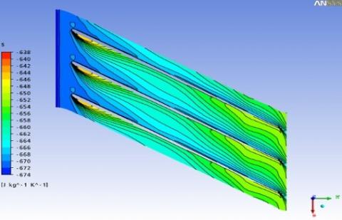
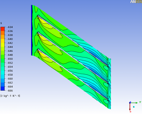
Figure 13. Entropy throughout the original impeller
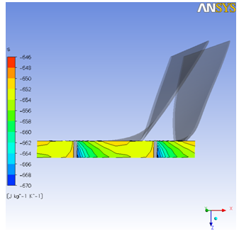
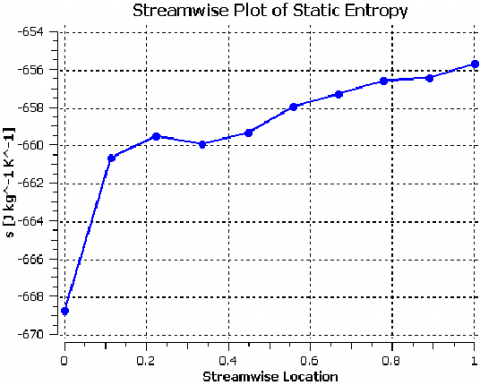
Figure 13 shows the average variation of entropy throughout the wheel. As it was so expected, entropy increases throughout the impeller, a time that true compression is not isentropic. Integrating this result in all the impeller, returning each point the value of the temperature and the mass, the CFX calculates the loss of overall efficiency. We can observe an increase in the entropy of the whole impeller. Represented on velocity figures. It is obvious that it is obtained at the CFX extract is the profile of the entropy by the whole impeller in positions of 20, 50 and 80% of the normal blade size. The figures produced will be shown to all to expose in detail where the greatest losses occur (Figures 14 to 16).
In Figure 14 a sample present in a region with a large loss of impeller output, possibly due to the formation of the mat and also the sliding of the blade, the entropy variation in all the walls of the impeller is due to a phenomenon turbulence.
Figure 15 sample that the variation of the entropy was more than what is in the previous figure. This means that the losses for the vortex and the mat if concentrated more in the crankcase area after the exit to the impeller.
Figure 16 shows the profile of the entropy in the impeller exit.
Figure 17 shows that the largest losses occur in the side of the blade pressure of the impeller and also in the next region to the crankcase, which corresponds to a normal blade size of 80%. These results are logical with the figures of the pressure, the number of absolute mach and the speed.
These are the results of the original impeller.
To optimize the impeller of this compressor and reduce turbulence losses, we have changed some parameters of the original man turbo impeller.
Figure 14. Entropy 20℅ of span. blade to blade
Figure 15. Entropy 50℅ of span. blade to blade
Figure 16. Entropy 80℅ of span. blade to blade
Figure 17. Entropy at the exit of the original impeller
5.2 Parametric study and optimization of the impeller
To show the validity of the correlations and models proposed in the study modifications have been made to the geometry of the compressor impeller. The main modified parameters correspond to the impeller: the axial length, the number of blades.
5.3 First optimization and parametric studies CFD
In this article the results to change the value of the axial length of the impeller will be displayed increased in more than 10 mm (Lax +), although to have if kept without changing, all the geometric parameters, had the change of the mesh because the format of the impeller has changed.
The data of the mesh are the following Table 6:
Table 6. Mesh data, impeller (Lax +)
|
Characteristics |
Total nodes |
Total element |
|
mesh |
48288 |
43060 |
Table 7 shows some execution parameters.
Table 7. Geometric parameters, impeller (Lax +)
|
input power (w) |
410718.0000 |
|
intake flow coefficient |
0.0123 |
|
outlet flow coefficient |
0.0913 |
|
total pressure ratio |
2.0041 |
|
total temperature ratio |
1.2374 |
|
isentropic efficiency |
92.6353 |
|
polytropic efficiency |
93.3213 |
The change in geometry of the shape to be increased in the distance between the inlet and the outlet of the impeller in the
meridian plane means that the bending of the impeller has been decreased.
It is so expected that this light results in increased friction losses and reduced losses due to turbulence phenomena mainly combines the formation of mats and internal recycling. Because the distance between the entrance and the exit will be greater, the format of blade theoretically, will be able to adapt better to the turbulent of the fluid.
Analyzing the two results it is verified that the modification of the geometry provided as a decrease in efficiency, that was for 92.63%. But the pressure reason is increased for 2.00, as the pressure reason is used for the calculation of efficiency, temperature and power. Figure 18 shows the variation of the average entropy throughout the impeller.
In Table 8 the mean values of some parameters in different positions of the domain are shown.
Table 8. Modified impeller parameter (Lax +)
|
Parameter |
Entrance |
Leading edge |
edge of leaks |
Exit |
|
Pstatic (pa) |
1675030.000 |
1673870.000 |
2482330.000 |
2590750.000 |
|
Ptotal (pa) |
1686780.000 |
1671170.000 |
3414630.000 |
3380430.000 |
|
Ptotal (rot) (pa) |
1675010.000 |
1661780.000 |
1597570.000 |
1592950.000 |
|
Tstatic (k) |
339.9550 |
339.4260 |
386.9860 |
391.9690 |
|
Ttotal (k) |
341.8260 |
341.7370 |
423.8920 |
422.9850 |
|
Ttotal (rot) (k) |
341.1180 |
341.0820 |
341.1530 |
341.1320 |
|
Enthalpy (J/kg) |
43157.1000 |
43121.2000 |
43192.4000 |
43170.8000 |
|
Entropy (J/kg) |
-670.0810 |
-667.8520 |
-656.4290 |
-655.6880 |
|
Mach abs |
0.1657 |
0.1993 |
0.6897 |
0.6283 |
|
Mach rel |
0.3430 |
0.3336 |
0.1522 |
0.2386 |
|
u (m/s) |
134.4650 |
134.3950 |
310.3170 |
333.5010 |
|
Cm(m/s) |
53.1702 |
58.9625 |
28.3206 |
26.8398 |
|
Cu (m/s) |
-47.2546 |
-75.9532 |
-273.2510 |
-244.5820 |
|
C (m/s) |
85.4879 |
108.1840 |
275.4330 |
246.4840 |
|
Wu (m/s) |
87.2106 |
58.4433 |
37.0672 |
88.9182 |
|
W (m/s) |
103.8120 |
87.5921 |
47.9239 |
94.0918 |
|
Flow Angle: Alpha |
-76.2488 |
-60.4858 |
61.1413 |
29.9624 |
|
Flow Angle: Beta |
-75.6264 |
-95.1815 |
-56.4439 |
-74.7556 |
Figure 18. Entropy throughout the modified Lax + impeller
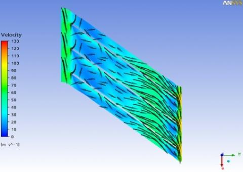
Figure 19. Velocity at span of 20℅, blade to blade
Figure 20. Velocity at span of 50℅, blade to blade
Figure 21. Velocity at the span of 80℅, blade to blade
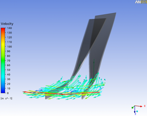
Figure 22. Chain Lines Speed. of impeller Lax +
Figure 23. Entropy 80, blade to blade
Comparing Figure 13 to Figure 18 we observe that the variation of entropy would be less than that in the original geometry man turbo. Clearly that this analysis is only qualitative, a period that it is necessary to determine the whole value of the losses to integrate in all the impeller the reason writes the variation of the entropy and the temperature. But in the original geometry, the entropy leaves a value of -669.25 J / kg. K and goes from stops -656.25 J / kg. K. For the case with the modified Lax + geometry that the whole variation of the entropy is clearly less, therefore goes from -668.75 J / kg. K to -655.75 / kg. K.
Comparing Table 8 and Table 5, we observe that the increased value of absolute machs of 0.6838 in the edge of leaks for 0.6897. Soon, the hypothesis that losses due to turbulence decrease is verified with these results. The evidence of this can be seen in Figures 19 to 23.
Figures 19 to 23 that the effect of the mat separation in the losses of the impeller is less than that in the original geometry. He can observe that the value of the velocity is lesse for the value in the original case (Figure 21). As it was so expected, there is a variation of entropy in the region where the mats are formed. This was not clearly seen in Figure 23 of the Lax + geometry. Because a small variation of the entropy in the original case.
If the result shows a decrease in efficiency concludes that the reduction in losses due to turbulence phenomena exceeds the increase in friction losses, although not having to get the reason for the expected pressure. Another explanation for decreased efficiency is the increase in the number of mach, the region that this leads to a decrease in efficiency.
Table 9 shows the result of Lax + optimized geometry, compared to the original geometry.
Table 9. Original impeller settings and modified impeller. (Lax +)
|
parameters |
original geometry |
geometry lax + |
percentage |
|
RP |
1.9948 |
2.0041 |
0.466 % |
|
RT |
1.2354 |
1.2374 |
0.161% |
|
η is (%) |
92.7412 |
92.6353 |
-0.114 % |
|
η pol (%) |
93.4136 |
93.3213 |
-0.098 % |
|
Power (w) |
407336.0000 |
410718.0000 |
0.830 % |
The data of the mesh are the following Table 10:
Table 10. Mesh data , impeller (Lax -)
|
Characteristics |
Total nodes |
Total element |
|
mesh |
44848 |
39956 |
Table 11 shows some execution parameters.
In Table 12, the average values of some parameters in different positions of the domain are shown.
Table 13 shows comparison of modified geometry Lax - results with original geometry.
Expected Result:
• Reduced friction.
• Increased turbulence.
Table 11. Geometric parameters, impeller (Lax -)
|
input power (w) |
404426.0000 |
|
intake flow coefficient |
0.0123 |
|
outlet flow coefficient |
0.0909 |
|
total pressure ratio |
1.9917 |
|
total temperature ratio |
1.2337 |
|
isentropic efficiency |
93.2141 |
|
polytropic efficiency |
93.8421 |
Table 12. Modified impeller parameter (Lax -)
|
Parameter |
Entrance |
Leading edge |
edge of leaks |
Exit |
|
Pstatic (pa) |
1675930.000 |
1675480.000 |
2490080.000 |
2594920.000 |
|
Ptotal (pa) |
1687200.000 |
1670620.000 |
3394890.000 |
3360380.000 |
|
Ptotal (rot) (pa) |
1675510.000 |
1661760.000 |
1607470.0000 |
1601360.000 |
|
Tstatic (k) |
339.9490 |
339.6430 |
386.7000 |
391.5810 |
|
Ttotal (k) |
341.8230 |
341.7180 |
422.5150 |
421.6930 |
|
T total (rot) (k) |
341.1210 |
341.0990 |
341.2120 |
341.1850 |
|
Enthalpy (J/kg) |
43159.8000 |
43138.1000 |
43251.8000 |
43224.4000 |
|
Entropy (J/kg) |
-670.1630 |
-667.8090 |
-658.0100 |
-657.0340 |
|
Mach abs |
0.1657 |
0.1907 |
0.6792 |
0.6190 |
|
Mach rel |
0.3445 |
0.3319 |
0.1622 |
0.2495 |
|
u (m/s) |
134.7340 |
134.4320 |
310.4010 |
333.5010 |
|
Cm(m/s) |
53.3209 |
56.3735 |
28.2137 |
26.8281 |
|
Cu (m/s) |
-47.6795 |
-72.4668 |
-270.9310 |
-239.7550 |
|
C (m/s) |
86.1794 |
104.1970 |
273.2000 |
241.7420 |
|
Wu (m/s) |
|
61.9670 |
39.4713 |
93.7461 |
|
W (m/s) |
103.9120 |
87.3359 |
49.6590 |
98.8533 |
|
Flow Angle: Alpha |
75.4021 |
-61.6495 |
77.1147 |
26.9968 |
|
Flow Angle: Beta |
75.3416 |
-92.4634 |
-57.2096 |
-75.4411 |
5.4 Second optimization and parametric studies CFD
Change the value of the axial length of the turbo man impeller will be displayed in less than 10 mm Lax-. Although to have if kept without changing the geometrical parameter, had the change of the mesh because the format of the impeller has changed.
The reason for pressure is decreasing for 1.9917, the pressure reason is used for the calculation of efficiency, temperature and power. We verify that these results are much better than the previous case analyzed.
Figure 24 shows the variation of the entropy throughout the impeller. Comparing Figure 24 to Figure 13 we observe that the variation of entropy in this case would be more than what in the original geometry. It is clear that this analysis is only qualitative, a period that it is necessary to determine the full value of losses to integrate throughout the impeller. But in the original geometry the entropy leaves a value of -669.25J / kg. K and it goes up to -656.25 J / kg. K. For the case with the modified geometry Lax- that all the variation of the entropy is clearly more, goes thus of -669 J / kg. K up to -657 J / kg. K.
The distance between the entry and the exit is less, the format of blade theoretically, will be able to increase the turbulence of the fluid.
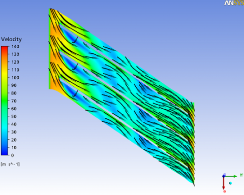
Comparing Table 12 and Table 5 it is observed that the value of absolute mach decreases by 0.6838 in the edge of leak for 0.6792. One possible explanation for the reduction in mach number that occurs, an increase in turbulence losses is that the transfer of rotor energy to the fluid is less because of little passage through the entire impeller. The evidence of this can be seen in Figures 25 to 28 a moment that velocitys are in this case also more.
Table 13. Original impeller settings and modified impeller. (Lax -)
|
parameters |
original geometry |
geometry lax- |
percentage |
|
RP |
1.9948 |
1.9917 |
-0.155% |
|
RT |
1.2354 |
1.2337 |
-0.137% |
|
η is (%) |
92.7412 |
93.2141 |
0.509% |
|
η pol (%) |
93.4136 |
93.8421 |
0.458% |
|
Power (w) |
407336.0000 |
404426.0000 |
-0.714% |
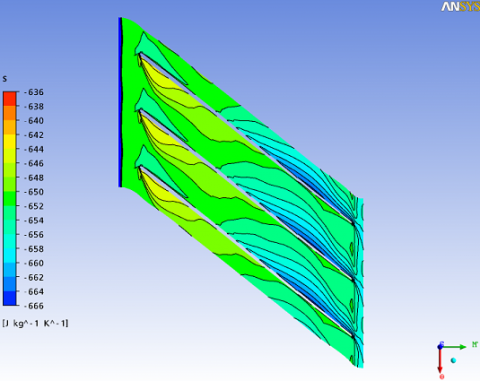
Figure 24. Entropy throughout the modified Lax- impeller
Figure 25. Velocity at span of 20℅, blade to blade
Figure 26. Velocity at span of 50℅, blade to blade
Figure 27. Velocity at the span of 80℅, blade to blade
Figure 28. Entropy 80℅ span. blade to blade
Figures 25 and 28 the effect of the mat in the losses of the impeller is more than what in the original geometry. He can observe that the maximum value of the Velocity is increased from 160 to 170 m / s. in the previous case, this velocity has reached a maximum value of 170 m / s. a more energy transfer occurs for the fluid, which it does with that to the influence of the losses for turbulence is more.
Figure 28 shows the entropy in the size of 80% span.
Expected Result:
• Reduced friction.
• Increased turbulence.
5.5 Final optimization of the impeller
5.5.1 Description of the final geometry
The same original impeller will be displayed but with 20 blades, although to have if kept all the geometrical parameters, had the change of the mesh because the number of blades has increased.
The data of the mesh (Table 14) are the following:
Table 14. Mesh data, impeller (20 blades)
|
Characteristics |
Total nodes |
Total element |
|
mesh |
34797 |
30388 |
Table 15 shows some execution parameters.
Table 15. Geometric parameters, impeller (20 blades)
|
input power (w) |
451067.0000 |
|
intake flow coefficient |
0.0138 |
|
outlet flow coefficient |
0.0998 |
|
total pressure ratio |
1.9926 |
|
total temperature ratio |
1.2344 |
|
isentropic efficiency |
92.9961 |
|
polytropic efficiency |
93.6449 |
The change in geometry increases the number of blades probably takes an increase in friction losses and greater losses for the gas incident. Therefore, it is expected that this slight change in friction loss and loss reduction increases due to the formation of mats and the internal recycling and reduction of the slip of the impeller output. If the result shows an increase in efficiency of 92.74% in the original geometry for 92.99%, concludes that the reduction of losses due to turbulence phenomena and slip surpasses the increase in friction losses. It can be seen that the pressure reason is decreasing for 1.9926.
Figure 29 shows the variation of the average entropy throughout the final impeller.
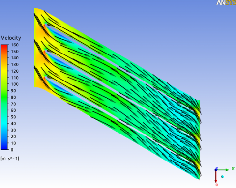
Comparing the value of the absolute mach of the base of case with this one, one observes a reduction of 0.6838 of the edge of fuit for 0.6827, with this fact one proves the reduction of the losses for the turbulence, thus the reduction of the velocity of the exit impeller exists. This always reinforces the hypothesis of the main cause of improvement in efficiency is because the compressor no longer meets in the clutter. We can see from Figures 30 to 33 the evidence of this is that the velocitys are in this case less.
Figures 30 To 33 that the effect of the mat in the impeller losses is less than what in the original geometry. It can be seen that the maximum value of the velocity has fallen from 130 to 120 m / s in 80% of the blade size.
In Table 16, the average values of some parameters in different positions of the domain are shown
Differently from the cases of change of impeller geometry, in which the fall of the velocity more was accentuated, in this case the fall was probably less being this the explanation of that increases of the efficiency.
In Figure 33 also it is possible to visualize a variation of the entropy in the region where the mats are formed. If the result shows an increase in efficiency concludes that the reduction of losses for turbulence and slip surpasses the increase in friction loss. It is observed that, the number of mach has come close to 0.72. apparently being a good result comparison with the original geometry and all the simulations. The sufficiently interesting data to be observed are the average value of absolute speed in the output of the impeller given in the form of Tables 5 and 16, in the original impeller the velocity is 244.93m / s, whereas in this case it is 243.54 m / s. therefore the absolute speed is decreased by comparing to that of the original geometry.
Differently from the cases of change of impeller geometry, in which the fall of the velocity more was accentuated, in this case the fall was probably less being this the explanation of that increases of the efficiency.
In Figure 33 also it is possible to visualize a variation of the entropy in the region where the mats are formed. If the result shows an increase in efficiency concludes that the reduction of losses for turbulence and slip surpasses the increase in friction loss. It is observed that, the number of mach has come close to 0.72. apparently being a good result comparison with the original geometry and all the simulations. The sufficiently interesting data to be observed are the average value of absolute speed in the output of the impeller given in the form of Tables 4 and 14, in the original impeller the velocity is 244.93m / s, whereas in this case it is 243.54 m / s. therefore the absolute speed is decreased by comparing to that of the original geometry.
Table 17 shows the comparison of results with original geometry.
Table 16. Modified impeller parameter (20 blades)
|
Parameter |
Entrance |
Leading edge |
edge of leaks |
Exit |
|
Pstatic (pa) |
1663710.000 |
1665490.000 |
2477020.000 |
2584510.000 |
|
Ptotal (pa) |
1683560.000 |
1673100.000 |
3388360.000 |
3354640.000 |
|
Ptotal (rot) (pa) |
1670950.000 |
1662780.000 |
1599870.000 |
1594230.000 |
|
Tstatic (k) |
339.5320 |
339.1900 |
386.5860 |
391.6020 |
|
Ttotal (k) |
341.8300 |
341.7000 |
422.7470 |
421.9460 |
|
T total (rot) (k) |
341.0670 |
341.0270 |
341.1240 |
341.1240 |
|
Enthalpy (J/kg) |
43106.2000 |
43065.6000 |
43162.6000 |
43163.1000 |
|
Entropy (J/kg) |
-669.5160 |
-668.1970 |
-656.9120 |
-655.9330 |
|
Mach abs |
0.1837 |
0.2016 |
0.6827 |
0.6213 |
|
Mach rel |
0.3515 |
0.3439 |
0.1642 |
0.2472 |
|
u (m/s) |
134.5440 |
134.3140 |
310.3640 |
333.5010 |
|
Cm(m/s) |
58.7362 |
58.3039 |
30.9744 |
28.4071 |
|
Cu (m/s) |
48.2326 |
-69.5816 |
-271.4370 |
-241.3880 |
|
C (m/s) |
91.0018 |
104.8130 |
274.0860 |
243.5460 |
|
Wu (m/s) |
86.3112 |
64.7341 |
38.9288 |
92.1133 |
|
W (m/s) |
106.2320 |
90.6905 |
50.9149 |
97.7586 |
|
Flow Angle: Alpha |
-76.7953 |
-64.2838 |
69.6999 |
40.4411 |
|
Flow Angle: Beta |
-76.1466 |
-91.8430 |
-54.7798 |
-73.4779 |
Figure 29. The entropy throughout the final impeller
Figure 30. Velocity at span of 20℅, blade to blade
Figure 31. Velocity at span of 50℅, blade to blade
Figure 32. Velocity at the span of 80℅, blade to blade
Figure 33. Entropy 80℅ span, blade to blade
Table 17. Original impeller settings and modified impeller. (20 blades)
|
parameters |
original geometry |
Geometry 20blades |
percentage |
|
RP |
1.9948 |
1.9926 |
-0.110 % |
|
RT |
1.2354 |
1.2344 |
-0.080 % |
|
η is (%) |
92.7412 |
92.9961 |
0.274 % |
|
η pol (%) |
93.4136 |
93.6449 |
0.247 % |
|
Power (w) |
407336.0000 |
451067.0000 |
10.735% |
The main limitation of the approach presented in this article is aerodynamic performance. For this, we used an approach based on the reduction of the sources internal to the impeller (it is the object of a selection of the aerodynamic parameters according to the acoustic computations), and using the software ANSYS CFX and the method k - ε.
For the nominal performance, we applied the criteria suggested by the literature, the main differences between the original impeller and the optimized one being the value of the slowdown. To check the aerodynamic profile of the centrifugal compressor impeller blades, we must change the impeller dimensions and focus on changing the axial length, but by changing the numbers of the blades, we obtain good results.
[1] Aungier, R.H. (2000). Centrifugal compressors: A strategy for aerodynamics design and analysis. ASME, New York, USA. https://doi.org/10.1115/1.800938
[2] Xu, C., Amano, R.S. (2008). Computational analysis of swept compressor rotor blades. International Journal for Computational Methods in Engineering Science and Mechanics, 9(6): 374-382. https://doi.org/10.1080/15502280802365840
[3] Xu, C., Amano, R.S. (2010). Computational analysis of scroll tongue shape to compressor performance by using different turbulence models. International Journal for Computational Methods in Engineering Science and Mechanics, 11(2): 85-99. https://doi.org/10.1080/15502280903563517
[4] Xu, C., Yang, H.Q., Jiang, Y.D., Yi, Z.W. (2019). The development of an integrally geared centrifugal compressor. International Journal of Fluid Mechanics & Thermal Sciences, 5(1): 1-9. https://doi.org/10.11648/j.ijfmts.20190501.11
[5] Xu, C. (2007). Design experience and considerations for centrifugal compressor development. Journal of Aerospace Engineering, 221(2): 273-287. https://doi.org/10.1243/09544100JAERO103
[6] Xu, C., Amano, R.S. (2012). Empirical design considerations for industrial centrifugal compressors. International Journal of Rotating Machinery, 2012. https://doi.org/10.1155/2012/184061
[7] Xu, C., Amano, R.S. (2009). Development of a low flow coefficient single stage centrifugal compressor. International Journal for Computational Methods in Engineering Science and Mechanics, 10(4): 282-289. https://doi.org/10.1080/15502280902939460
[8] Xu, C., Amano, R.S. (2009). The development of a centrifugal compressor impeller. International Journal for Computational Methods in Engineering Science and Mechanics, 10(4): 290-301. https://doi.org/10.1080/15502280903023165
[9] Xu, C., Amano, R.S. (2010). Study of the flow in a centrifugal compressor. International Journal of Fluid Machinery and System, 3(3): 260-270. https://doi.org/10.5293/IJFMS.2010.3.3.260
[10] Turner, M.G., Merchant, A., Bruna, D. (2006). A turbomachinery design tool for teaching concepts for axial-flow fans, compressor, and turbines. ASME Turbo Expo 2006: Power for Land, Sea, 1: 937-952. https://doi.org/10.1115/GT2006-90105
[11] Xu, C., Amano, R.S. (2009). On the development of turbomachine blade aerodynamic design system. International Journal for Computational Methods in Engineering Science and Mech, 10(3): 186-196. https://doi.org/10.1080/15502280902795052
[12] Cohen, H., Rogers, G.F.C., Saravanamutto, H.I.H. (1996) Gas Turbine Theory. Pearson, New York.
[13] Rangwala, A.S. (2005). Turbo-Machinery Dynamics. Design and Operation, McGraw-Hill, USA.
[14] Niazi, S., Stein, A., Sankar, L.N. (2000). Numerical studies of stall and surge alleviation in a high-speed transonic fan rotor. AIAA, pp. 2000-0225. https://doi.org/10.2514/6.2000-225
[15] Aghaei Tog, R., Mesgharpoor Tousi, A., Soltani, M. (2007). Design and CFD analysis of centrifugal compressor for a microgasturbine. Aircraft Engineering and Aerospace Technology, 79(2): 137-143. https://doi.org/10.1108/00022660710732680
[16] Xu, C., Muller, M. (2005). Development and design of a centrifugal compressor volute. Int. J. Rotating Machinery, 3: 190-196. https://doi.org/10.1155/IJRM.2005.190
[17] Yutaka, O., Takashi, G., Eisuke, O. Effect of tapered diffuser vane on the flow field and noise of a centrifugal compressor. Journal of Thermal Science, 16(4): 301-308. https://doi.org/10.1007/s11630-007-0301-1
[18] Ling, J., Wong, K.C., Armfeild, S. (2007). Numerical investigation of a small gas turbine compressor. 16th Australian Fluid Mechanics Conference, Crown Plaza, Gold Coast, Australia, 2-7.
[19] Shu, X.W., Gu, C.G., Xiao, J., Gao, C. (2008). Centrifugal compressor blade optimization based on uniform design and genetic algorithm. Frontiers of Energy and Power Engineering, p. 453. https://doi.org/10.1007/s11708-008-0083-5
[20] Tang, J., Turunen-Saaresti, T., Larjola, J. (2008). Use of partially shrouded impeller in a small centrifugal compressor. Journal of Thermal Science, 17(1): 21-27. https://doi.org/10.1007/s11630-008-0021-1
[21] Shaaban, S. (2015). Design optimization of a centrifugal compressor vaneless diffuser. International Journal of Refrigeration, 60: 142-154. https://doi.org/10.1016/j.ijrefrig.2015.06.020
[22] Kim, C., Lee, H., Yang, J., Son, C., Hwang, Y. (2016). Study on the performance of a centrifugal compressor considering running tip clearance. International Journal of Refrigeration, 65: 92-102. https://doi.org/10.1016/j.ijrefrig.2015.11.008
[23] Pischinger, S., SchQnfelder, C., Bornscheuer, W., Kindl, H., Wiartalla, A. (2001). Integrated air supply and humidification concepts for fuel cell systems. SAE International, Warrendale, PA. https://doi.org/10.4271/2001-01-0233
[24] Xu, C., Amano, R.S. (2008). Computational analysis of swept compressor rotor blades. International Journal for Computational Methods in Engineering Science and Mechanics, 9(6): 374-382. https://doi.org/10.1080/15502280802365840
[25] Xu, C., Amano, R.S. (2017). Effects of asymmetric radial clearance on performance of a centrifugal compressor. Journal of Energy Resources Technology, 140(5). https://doi.org/10.1115/1.4038387
[26] Xu, C., Amano, R.S. (2017). Centrifugal compressor performance improvements through impeller splitter location. Journal of Energy Resources Technology, 140(5). https://doi.org/10.1115/1.4037813
[27] Gonzalez, J., Fernandez, J., Blanco, E., Santolaria, C. (2002). Numerical simulation of dynamic effects due to impeller-volute interaction in a centrifugal pump. Journal of Fluids Engineering, 124(2): 348-355. https://doi.org/10.1115/1.1457452
[28] Chima, R.V. (2006). A three-dimensional unsteady CFD model of compressor stability. ASME Turbo Expo 2006, 6: 1157-1168. https://doi.org/10.1115/GT2006-90040
[29] Denton, J.D., Dawes, W.N. (1998). Computational fluid dynamics for turbomachinery design. Journal of Mechanical Engineering Science, 213(2): 107-124. https://doi.org/10.1243/0954406991522211
[30] Dickmann, H.P., Wimmel, T.S., Szwedowicz, J., Filsinger, D., Roduner, C.H. (2006). Unsteady flow in a turbocharger centrifugal compressor, three-dimensional computational fluid dynamics simulation and numerical and experimental analysis of impeller blade vibration. Journal of Turbomachinery, 128(3): 455-465. https://doi.org/10.1115/1.2183317
[31] Xu, C., Amano, R.S. (2012). Aerodynamic and structure considerations in centrifugal compressor design-blade lean effects. Turbo Expo, pp. 557-568. https://doi.org/10.1115/GT2012-68207
[32] Japikse, D. (1996). Centrifugal Compressor Design. Concepts, ETI Inc. Norwich, Vermont, 3rd edition.