Mariusz Ciesielski* | Jarosław Siedlecki | Maciej K. Janik
© 2020 IIETA. This article is published by IIETA and is licensed under the CC BY 4.0 license (http://creativecommons.org/licenses/by/4.0/).
OPEN ACCESS
In this paper, the mathematical model of the electrical and thermal processes proceeding during the electrosurgical polypectomy is considered. During a colonoscopy, the endoscopist can remove abnormal growths (polyps) inside the large intestine (the colon). In the electrosurgical polypectomy procedure, a polypectomy snare is tightened around the base of the polyp. Next, the electric current flows for a short moment of time from the snare loop (the first electrode), through the polyp-colon tissues and the other body tissues, to the second electrode placed on the patient’s skin. Both electrodes are connected to the electrosurgical generator unit. This medical surgery allows to cut off the polyp stalk from the colon wall. The systems of the partial differential equations that describe the thermal and electrical processes with the appropriate initial-boundary conditions are proposed. The examples of numerical simulations related to two duty cycles of the electrosurgical generator unit are presented. Simulation results can be helpful for the surgeons to choose the optimal heating time and to set other parameters of the electric current that flows by tissues during the endoscopy procedure.
electrosurgical polypectomy, Pennes bio-heat transfer model, biological tissue heating, tumor
Colon polyps are slow-growing growths (tumors) generally arising in the large intestine (colon). Colorectal cancer is one of the most common cancers with a very high mortality rate and can be treated as an important medical problem. One of the methods of treatment is a colonoscopic polypectomy [1, 2] that involves the prevention of colorectal cancer. The polypectomy is an invasive method of treatment. The beginnings of this method date back to the 1969 (performed by Shinya and Ichikawa). Many polyps discovered in the colonoscopic examination can be removed directly or biopsied. Knowledge of the characteristics of endoscopic instruments and accessories, and the geometry and size of the polyp is a very important for the proper removal of polyps by an experienced surgeon.
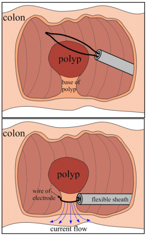
Most polyps can be removed using different polypectomy methods [3-5], but the most frequently used method of examination is the electrosurgical polypectomy. In this procedure, a polypectomy snare (wire loop) is passed over the base of the polyp and tightened around the polyp. The snares used in the colonoscopic polypectomy are made from different materials (the most often are made from the braided stainless-steel wire) and are available in a variety of sizes (typically 0.3-0.5mm in diameter) and in shapes of a continuous wire loop (typically 2.0-2.5cm in diameter). The snares are placed within a flexible sheath which is passed through the accessory channel of the colonoscope (a channel size is of 3-5mm and length is about 2.5m). The wire and sheath are connected to the moving plastic handle at the end of the device controlled by the surgeon. The handle allows the opening and closing of the wire loop. Additionally, the handle contains an electrical connector which couples the snare wire with an active cord to the electrosurgical unit (generator). The most popular approach for the considered application in this work are the monopolar snares. In this case, a high frequency (between 300 kHz and 1 MHz) electrical current is delivered for a very short period of time from the electrosurgical generator unit to the wire loop (the first electrode). Next, the current flows through the polyp-colon tissues (being in contact with the wire loop) and other body tissues to a remote return electrode (the grounding pad) placed e.g. on the patient’s back and returns to the electrosurgical generator unit completing the circuit. The electrical current has the highest concentration in the tissue near the contact with the wire loop, while it travels to the large surface area dispersive electrode through the body tissues with lower concentrations. In Figure 1, one can see the scheme of surgical operation in polypectomy.
The passage of an electric current through biological tissues generates heat (local thermal energy) which, in consequence, the temperature within tissues must increase (in order to occur a protein denaturation and next, to obtain a coagulation) [6-8]. It can be noted here that the electrocautery should take place, which causes the closing of the wound and the stopping of the bleeding – then the polyp is cut off from the colon wall. In the process of thermal coagulation, the tissue destruction occurs if the temperature within the tissue increases to approximately 60℃. The thermal coagulation causes the changes in the structure of the biological tissues. The temperature should only rise within the target tissue, preferably within the base of the polyp and any thermal damage of tissues (especially the intestinal tissue) must be avoided, because this can lead, for instance, to colon perforation. Also, when the electric current has stopped, hot tissues cause the further dissipation heating within the adjacent tissues. From the polypectomy treatment point of view, these recommendations are very important during polypectomy.
Figure 1. Scheme of surgical operation in polypectomy
In this paper, the authors commenced the development of the mathematical model and conducted the exemplary computational simulations related to the above-described problems. The main aim of this work is research that deals with the determination of the spatial transient-state temperature distribution and thermal damage of tissues in the polyp-colon system. The geometry of typical shape of the polyp with the considered part of the colon can be treated as an axially-symmetrical domain. Two different duty cycles of the electric current flow during the electrosurgical polypectomy in simulations are analyzed. The duty cycle refers to the percentage of total time in which the electrical current is actually delivered to the tissues.
The mathematical models describing heat transfer proceedings in the vital tissues are usually based on the most popular Pennes equation [9-15] and this approach has been adopted to modeling of heat transfer processes proceeding in the polyp-colon system. The typical Pennes equation contains two terms (heat sources) associated with the blood perfusion and metabolism in tissues. The heat transfer model in the wire loop is based on the Fourier-Kirchhoff equation. The wire loop is the first electrode, while the second (ground) electrode is usually placed on the skin of the patient’s back. If such a system will be considered, then the geometric model becomes too complicated. In order to simplify the model, it is assumed that the ground potential on the outer surface of colon is taken into account, while simultaneously the smaller difference of electric potentials between the first electrode and the surface of colon is assumed. During the electric current flow through tissues, the stationary electric potential distribution in the tissue domains should be determined considered the adequate boundary conditions. When the electric current flows through tissues, electric energy is converted to heat (the Joule heating effect). The heat source generation rate depends on the gradient of the electric field potential. Next, the heat source is introduced into the Pennes equation as an additional term (causing the tissues heating and eventually, their thermal damage). The process of heat generation in tissues ends when the electric current stops flowing. It should be pointed out that heat is still transferred from the warmer parts of the tissues to the adjacent sections of tissues which may cause their further damage. To determine the degree of the tissue damage, the Arrhenius damage integral is calculated [16-19].
The proposed mathematical model is solved using the numerical methods, because the analytical solution of equations of the mathematical model seems to be impossible especially for the complex geometry of the considered polyp-colon domain. For this purpose, the authors applied the Control Volume Method – CVM (known also in literature as the Finite Volume Method – FVM), while the Voronoi tessellation [20, 21] has been used in discretization of the considered domain. This selected numerical method is a well-known by the authors and has been used many times to solve other problems – e.g. [22]. It can be noted that other computational methods (e.g. the Finite Element Method – FEM [23, 24]) can be used to solve the mathematical model.
The remainder of this paper is structured as follows: Section 2 presents the mathematical model containing the description of the domain’s geometry, the governing equations for heat transfer in the particular sub-domains with the boundary and initial conditions, the governing equations of the electric field in the tissue sub-domains with the boundary conditions, definition of the heat source related to the Joule heating effect and definition of the Arrhenius damage integral. In Section 3, the description of numerical simulations (including discretization of sub-domains, all thermophysical parameters of sub-domains and other data) is given and also many illustrative simulation results are presented. The conclusions are provided in Section 4 of this article.
The considered domain consists of the following three sub-domains:
W1 - the colon tissue,
W2 - the polyp tissue (tumor),
W3 - the steel wire loop electrode.
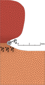
The geometrical model of this domain (as the axially symmetrical object) is presented in Figure 2. The outer surface limiting the domain (boundaries $\Gamma_{b 1}$, $\Gamma_{b 2}$ and $\Gamma_{b 3}$) is in contact with environment (i.e. a gas inside the colon). The boundaries denoted by $\Gamma_{k-l}$, where (k-l) $\in$ {(1-2), (1-3), (2-3)}, are the interfacial surfaces between adjacent sub-domains. The boundary $\Gamma_{z}$ is a part of the outer surface of the colon, while the boundary $\Gamma_{0}$ denotes the ‘virtual cutting surface’ of the colon wall and the boundary $\Gamma_{r}$ is on the symmetry axis.
Figure 2. The considered domain of the polyp-colon system (longitudinal section as the 2D domain)
2.1 Bio-heat transfer model
The temperature field in the considered domain (in the 2D cylindrical axis-symmetrical coordinates system) is described by the following system of equations
$(r, z) \in \Omega_{m}: \quad c_{m}(T) \rho_{m}(T) \frac{\partial T_{m}(r, z, t)}{\partial t}$$=\frac{1}{r} \frac{\partial}{\partial r}\left(r \lambda_{m}(T) \frac{\partial T_{m}(r, z, t)}{\partial r}\right)+$$\frac{\partial}{\partial z}\left(\lambda_{m}(T) \frac{\partial T_{m}(r, z, t)}{\partial z}\right)$$+Q_{m}(r, z, t)+Q_{\text {elect } m}(r, z, t)$ (1)
where, sub-index m = 1,2,3 identifies the particular sub-domains (as mentioned above), T [℃] is the temperature, (r, z) [m], t [s] denote two-dimensional cylindrical coordinates and time, c [J/(kg K)], r [kg/m3], $\lambda$ [W/(m K)] are the specific heat, the density and the thermal conductivity, respectively.
In the system of equations (1), the terms Qm [W/m3], for m = 1, 2, 3, are the capacities of volumetric internal heat sources associated with the blood perfusion and metabolic heat in tissues. The tissues in $\Omega_{1}$ and $\Omega_{2}$ are fed by a large number of uniformly spaced capillary blood vessels, hence the Pennes model can be used
$Q_{m}(r, z, t)$$=\left\{\begin{array}{ll}Q_{\text {met } m}+c_{\text {blood }} \rho_{\text {blood }} G_{\text {blood } m}\left[T_{\text {blood }}-T_{m}(r, z, t)\right], & m=1,2 \\ 0 & m=3\end{array}\right.$ (2)
where, Gbloodis the blood perfusion rate in the tissue [m3(blood)/(s m3(tissue))], $\rho_{\text {blood }}$ is the blood specific heat, rblood is the blood density and Tblood is the average blood temperature in the human body. The metabolic heat source Qmetcan be treated as a temperature-dependent function Qmet≡ Qmet(T(r,z,t)) or a constant value.
Eq. (1) is supplemented by the set of initial-boundary conditions. For t=0, the initial condition is given as
$\left.T_{m}(r, z, t)\right|_{t=0}=T_{i n t}, \quad m=1,2,3$ (3)
Here, one can assume that the initial temperature Tinit is equal to the average temperature Ttissue of the human body. On the contact surfaces between all sub-domains, the continuity conditions are assumed
$(r, z) \in \Gamma_{k-l}:$$\left\{\begin{array}{c}-\lambda_{k} \frac{\partial T_{k}(r, z, t)}{\partial n}=-\lambda_{l} \frac{\partial T_{l}(r, z, t)}{\partial n} \\ T_{k}(r, z, t)=T_{l}(r, z, t)\end{array}\right.$ (4)
where, (k-l) $\in$ {(1-2), (1-3), (2-3)} and the operator $\partial / \partial n$ denotes a normal derivative. The non-flux boundary condition on the boundary $\Gamma_{r}$ is given
$(r, z) \in \Gamma_{r}:$$\left.\frac{\partial T_{m}(r, z, t)}{\partial r}\right|_{r=0}=0, \quad m=1,2$ (5)
On the external surfaces of the sub-domains, the Dirichlettype (on the boundaries $\Gamma_{0}$ and $\Gamma_{z}$ ) and the Robin-type (on the outer surfaces of the sub-domains: $\Gamma_{b 1}, \Gamma_{b 2}$ and $\Gamma_{b 3}$ ) boundary conditions are assumed
$(r, z) \in\left\{\Gamma_{0}, \Gamma_{z}\right\}: \quad T_{1}(r, z, t)=T_{\text {tissue }}$ (6)
$(r, z) \in \Gamma_{b m}:-\lambda_{m} \frac{\partial T_{m}(r, z, t)}{\partial n}=\alpha_{m}\left[T_{m}(r, z, t)-T_{a m b}(t)\right]$ (7)
where, $\alpha_{m}$ [W/(m2 K)], for m = 1, 2, 3, are the convective heat transfer coefficients and Tamb [℃] can be treated as the gas temperature in the large intestine (colon) or Tamb.= Ttissue.
2.2 Electrical potential model
The electrical current flows in the period of time theating. The heat generation rate per unit volume Qelect inside the tissue sub-domains is related to the electric field (also called as the Joule heating effect)
$Q_{\text {elect } m}(r, z, t)=\left\{\begin{array}{ll}H(t) \sigma_{m}\left|\nabla \varphi_{m}(r, z)\right|^{2} & \text { if } m=1,2 \\ 0 & \text { if } m=3\end{array}\right.$$=\left\{\begin{array}{ll}H(t) \sigma_{m}\left[\left(\frac{\partial \varphi_{m}(r, z)}{\partial r}\right)^{2}+\left(\frac{\partial \varphi_{m}(r, z)}{\partial z}\right)^{2}\right] & \text { if } m=1,2 \\ 0 & \text { if } m=3\end{array}\right.$ (8)
where, $\varphi[\mathrm{V}]$ is the electrical potential, $\sigma$ [S/m] is the electrical conductivity and H(t) is the time-dependent function related to the duty cycle of the electrosurgical generator unit, and this function describes the current flow over time.
The electrical potential distribution in the tissue sub-domains results from solving the following system of equations [7, 25]
$(r, z) \in \Omega_{m}: \frac{1}{r} \frac{\partial}{\partial r}\left(r \sigma_{m} \frac{\partial \varphi_{m}(r, z)}{\partial r}\right)$$+\frac{\partial}{\partial z}\left(\sigma_{m} \frac{\partial \varphi_{m}(r, z)}{\partial z}\right)=0, \quad m=1,2$ (9)
with the boundary conditions governing the electric potential field. On the contact surfaces of the tissue sub-domains with the one of the electrodes (wire), the boundary condition is defined as
$(r, z) \in\left\{\Gamma_{1-3}, \Gamma_{2-3}\right\}: \quad \varphi_{m}(r, z)=U_{1}, \quad m=1,2$ (10)
where, U1 is the applied voltage on the wire loop electrode. As mentioned in the introduction, the real location of the second electrode is on the skin e.g. of the patient’s back. In this model, the direct influence of the ground electrode potential is simplified using the following assumption
$(r, z) \in\left\{\Gamma_{0}, \Gamma_{z}\right\}: \quad \varphi_{1}(r, z)=U_{2}$ (11)
Here, the average intermediate electrical potential U2 on the ‘virtual cutting surface’ of the colon wall is assumed. This should be clarified that the analysed part of the colon tissue is in ideal contact with other human tissues and is, in consequence, connected to the second electrode. The value of U2 = 0 also can be assumed, because the difference between the two electrode potentials U1 – U2 is essential in order to further calculate the value of the potential gradient.
Between both tissue sub-domains (the contact surface G1-2), the continuity condition is assumed
$(r, z) \in \Gamma_{1-2}:\left\{\begin{array}{c}\sigma_{1} \frac{\partial \varphi_{1}(r, z)}{\partial n}=\sigma_{2} \frac{\partial \varphi_{2}(r, z)}{\partial n} \\ \varphi_{1}(r, z)=\varphi_{2}(r, z)\end{array}\right.$ (12)
while on the boundaries of the analyzed domain that are not in contact with the wire electrode (the boundaries are electrically insulative), the following boundary condition is given:
$(r, z) \in\left\{\Gamma_{b 1}, \Gamma_{b 2}, \Gamma_{r}\right\}: \frac{\partial \varphi_{m}(r, z)}{\partial n}=0, \quad m=1,2$ (13)
2.3 Tissue damage model
The increase in the temperature of local tissue above a certain threshold will lead to irreversible cellular damage with interruption of the metabolic processes. Based on the knowledge of the spatio-temporal temperature distribution, one can determine the degree of the tissue damage. Under the assumption that the thermal damage of tissue (the tissue denaturation) is an irreversible process, the Arrhenius model [17-19] is applied. The Arrhenius damage integral is defined as:
$\Psi(r, z, t)=\int_{0}^{t} P \exp \left(-\frac{\Delta E}{R_{g} \cdot(T(r, z, \tau)+273)}\right) d \tau$ (14)
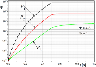
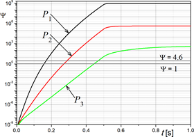
The values of this integral (mainly depending on the tissue temperature history at the selected point (r, z) of tissue) are compared with threshold values. The value of $\Psi$= 1 means a 63% probability of cell death at a specific point of the tissue domain, while the value of $\Psi$= 4.6 indicates that the thermal damage is almost complete (99% probability of cell death). In Eq. (14), P [1/s] is the pre-exponential factor, $\Delta E$ [J/mol] is the activation energy and Rg [J/(mol K)] is the universal gas constant. Achieving the appropriate threshold for tissue damage is important in regards to the patient’s safety during polypectomy. The tissue damage should be always limited to minimal one, and simultaneously, it must ensure success for medical procedure. Hence, the threshold for tissue damage should be also at a minimum level that ensures tissue damage.
Remark: The above introduced models: Biological heat transfer model, potential model and tissue damage model are coupled. At first, the electric potential field distribution satisfied the given boundary conditions in the considered domain is determined. Next, the values of the internal heat source in tissues related to the Joule heating are calculated on the basis of the gradient of the squared electric field. The solution of the system of heat transfer equations with the heat source term (the Joule heating) allows one to determine the spatio-temporal temperature distribution in the domain. Finally, the degree of the tissue damage is calculated on the basis of the value of the Arrhenius damage integral.
The partial differential equations of mathematical models (describing the thermal and electrical processes) presented in Section 2 have been solved numerically using the Control Volume Method. The details about this method one can find in our earlier papers [20-22].
The Voronoi discretisation of the considered colon-polyp domain is presented in Figure 3. Every control volume has the shape of a ring.
Figure 3. Discretisation of the considered polyp-colon domain into control volumes
The thermophysical parameters of particular sub-domains are following [26, 27]: $\lambda_{1}$=$\lambda_{2}$= 0.55 W/(m K) (for frequency f = 400 kHz), $\lambda_{3}$= 15 W/(m K), c1 = c2 = 1041 J/(kg K), c3 = 500 J/(kg K), cblood = 3650 J/(kg K), $\rho 1$= $\rho 2$ = 3655 kg/m3, $\rho 3$= 8000 kg/m3, $\rho_{\text {blood }}$= 1069 kg/m3, Gblood 1 = Gblood 2 = 0.538·10-3 s-1, Qmet 1 = Qmet 2 = 684 W/m3, $\sigma_{1}$=$\sigma_{2}$= 0.25 S/m, $\sigma_{3}$= 1.45·106 S/m, P = 3.1·1098 1/s, $\Delta E$= 6.27·105 J/mol, Rg = 8.314 J/(mol K). One can note that for both types of tissue: colon and polyp, the identical values of parameters have been assumed. The thermophysical parameters for the polyp are unknown in the literature, and the authors hold the opinion that the both values are very close. Also, the temperature-dependent parameters of every sub-domain can be used in the computations and from the numerical point of view, can be easily implemented. The remaining parameters used in simulation are the following: Tblood = 37℃, Tinit = 37℃, Tamb = 37℃, $\alpha_{1}$=$\alpha_{2}$=$\alpha_{3}$=10 W/(m2 K).
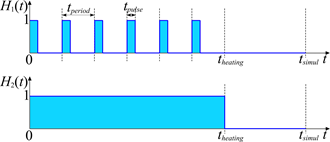
In this work, the following two functions H(t) describing the time-dependent electrical pulses are considered
Case 1:
$H_{1}(t)=\left\{\begin{array}{ll}1 & \text { if }\left\{t / t_{\text {period }}\right\} \leq t_{\text {pulse }} \wedge t \leq t_{\text {heating }} \\ 0 & \text { otherwise }\end{array}\right.$ (15)
Case 2:
$H_{2}(t)=\left\{\begin{array}{ll}1 & \text { if } t \leq t_{\text {heating }} \\ 0 & \text { otherwise }\end{array}\right.$ (16)
where, the time theating is the final moment of simulation time in which the flow of the electrical current through the wire electrode takes place, the time tsimul (≥ theating) is the total time of simulation. In Eq. (15), the time tpulse is the pulse duration time, while the operator {t/tperiod} returns the floating point remainder of dividing t by tperiod. In Figure 4, the courses of functions H(t) are presented schematically.
Figure 4. The courses of functions H1(t) and H2(t)
If the current is delivered continuously for the entire activation period (with no pauses in the interval [0, theating]), then it is defined as a 100% duty cycle. In the first case, the current with a duty cycle of tpulse / tperiod ·100% is taken into account.
3.1 Results for Case 1
In the first simulation, the additional parameters have been assumed: U1 – U2 = 120 V, tperiod = 0.025 s, tpulse = 0.005 s, theating = 0.5 s, tsimul = 1 s. Here, the duration of the current pulses corresponds to a 20% duty cycle.
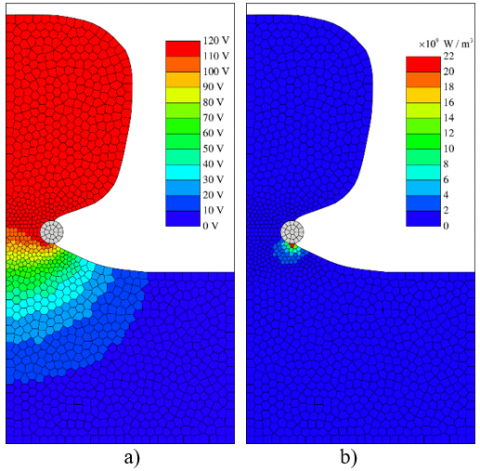
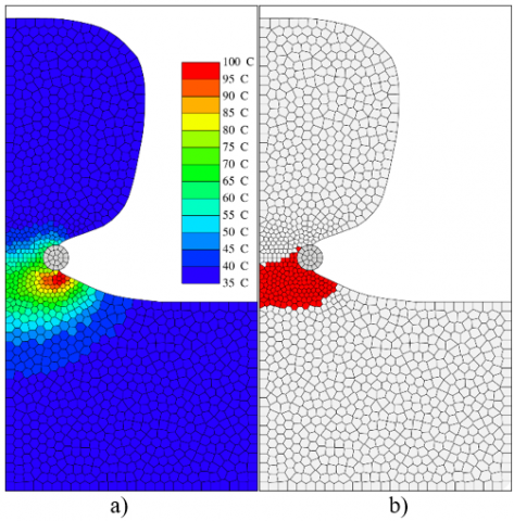
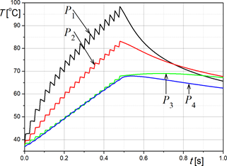
The electric potential distribution and the internal heat source distribution are presented in Figures 5a and 5b, respectively. The temperature field presented in Figure 6a shows the stage of heating tissues at theating = 0.5 s, while in Figure 6b the total tissue damage as the value of the Arrhenius damage integral $\Psi$ at tsimul = 1 s is presented. After the heating time theating = 0.5 s, the thermal diffusion process in the considered domain takes the place (heat in the selected part of tissues is slowly transferred to neighbouring tissues) and simultaneously the tissue damage process is still growing. The next two Figures 7 and 8 show the heating curves and the growth kinetics of the Arrhenius damage integral $\Psi$ over time, respectively, at the selected control volumes (marked in Figure 3) of tissue and wire electrode sub-domains.
Figure 5. a) Electric potential field distribution $\varphi$, b) internal heat source distribution $\sigma|\nabla \varphi|^{2}$ (Case 1)
Figure 6. Temperature distribution after theating = 0.5 s and the tissue damage (the values of the Arrhenius integral) after tsimul = 1 s (the red color of the control volumes denotes that $\Psi$> 4.6) (Case 1)
Figure 7. The heating curves at selected control volumes of tissue and wire electrode domains (see Figure 3) for theating = 0.5 s (Case 1)
Figure 8. The growth kinetics of the Arrhenius damage integral Y at selected control volumes of tissue domain (see Figure 3) for theating = 0.5 s (Case 1)
3.2 Results for Case 2
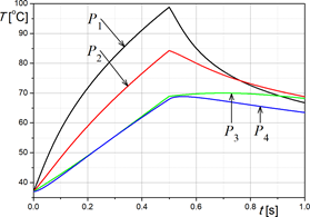
In this simulation, the lower difference between the two electrode potentials U1 – U2 = 55 V has been assumed. This value has been determined experimentally, in order to obtain a similar level of temperature rise in the tissues in the same time theating = 0.5 s (here, the current flows constantly in the interval [0, theating], 100% duty cycle). The remaining parameters used in this simulation are identical to these in the previous one. Figures 9-12 present numerical results of simulation - corresponding to the results for Case 1 presented in Figures 5-8.
Figure 9. a) Electric potential field distribution $\varphi$, b) internal heat source distribution $\sigma \mid \nabla \phi^{2}$ (Case 2)
In both cases of simulations, the parameters of the electrical current and heating times have been determined in such a way that the temperature in the tissue domains did not exceed the level of 100℃ and the zone of the tissue destruction in the base of the polyp was optimal (i.e. caused the least invasive for colon). Otherwise, temperature increases in the tissue sub-domains to a temperature greater than 100℃ caused the cellular water to boil and the cells to rupture. Modeling of such a process is omitted in this work (this will be the subject of further research). One can note that the temperature rise in tissues is the most intense during the current flow through biological tissues. The tissue damage still continues after the current flow through tissues is finished - it follows from the definition of the Arrhenius damage integral. Most of all, the tissue destruction depends on: the heating time, the history of tissue temperature over time, the assumed size and geometry of the polyp-tissue-wire system and the given electrical parameters. The shorter heating time may not cause the thermal damage of the base of the polyp and subsequently its cut off. The longer heating time can lead to the damage of larger tissue domain, and the perforation of the colon tissue may take place. Hence, it is very important to choose the suitable interval of the heating time. By comparing the results of both simulations (different the duty cycles are used), it can be concluded that the obtained results are similar.
Figure 10. Temperature distribution after theating = 0.5 s and the tissue damage (the values of the Arrhenius integral) after tsimul = 1 s (the red color of the control volumes denotes that $\Psi$ > 4.6) (Case 2)
Figure 11. The heating curves at selected control volumes of tissue and wire electrode domains (see Figure 3) for theating = 0.5 s (Case 2)
Figure 12. The growth kinetics of the Arrhenius damage integral $\Psi$ at selected control volumes of tissue domain (see: Figure 3) for theating = 0.5 s (Case 2)
This paper investigated the heat transfer problem during electrosurgical polypectomy. From the mathematical point of view, three models related to the thermal processes in the biological tissues and the wire electrode, the electrical potential model in the colon-polyp system and the tissue damage model have been proposed and considered. These models are conjugated together.
The mathematical model has been solved numerically using the Control Volume Method. The simplified polyp-colon domain has been discretized by the Voronoi tessellation (the 2D control volumes mesh). The advantage of the Voronoi tessellation is the rather accurate reconstruction of the shape of the particular sub-domains. Furthermore, the application of the Control Volume Method ensures a good approximation of the differential equations describing the thermal energy and electrical potential balances.
1. The considered problem, from the medical practice’s point of view, seems to be very interesting. We are aware that many doctors have little knowledge of the mathematical modeling of the physical processes discussed in this work.
2. The presented illustrative results in this work (among others, the distribution of temperature field in the tissues, the distribution of the tissue thermal damage) allow doctors to recognize and better understand the physical processes occurring during the electrosurgical polypectomy.
3. The endoscopist can apply the simulation results (performed individually for a specific case, of course) for to make the decision about the execution of the endoscopy procedure. The detailed knowledge of processes proceedings in the polyp-colon domain will allow for the appropriate choice of the optimal heating time and the optimal parameters of the electric current generated by the electrosurgical unit, depending on the geometry of the given polyp.
4. The construction of mathematical models for polypectomy seems to be highly needed for creating better and safer endoscopy procedures. Results of the numerical simulations may be helpful in the treatment strategy for clinical applications. We think that this scientific research will lead to a better treatment of the patients
The latest research and opinions [14, 15, 28, 29] related to the bio-heat transfer problems proceedings in the living biological tissues prove that the bio-heat models should be described by the non-Fourier heat conduction models, among others, by the modified Pennes equation derived from the Cattaneo-Vernotte model or from the dual phase lag model. In the Cattaneo-Vernotte model, the relaxation time appears, while in the second model, the thermalizaton time additionally occurs. In the future, we would like to apply these models in the mathematical modelling of heat transfer in related problems. The main difficulty is e.g. the lack (in the literature) of experimental data that determine the values of phase lag times for the colon (the large intestine) and polyp tissues. In the future, we also plan to carry out simulations for other types of polyps, to use the more complex shapes of the tissues, and to investigate the influence of other current parameters on the course of the polypectomy.
|
c |
specific heat, J kg-1 K-1 |
|
cblood |
blood specific heat, J kg-1 K-1 |
|
$\Delta E$ |
activation energy, J mol-1 |
|
Gblood |
blood perfusion rate in the tissues, m3(blood) s-1 m-3(tissue) |
|
H |
function describing the time-dependent rectangular electrical pulses |
|
$\partial / \partial n$ |
normal derivative |
|
P |
pre-exponential factor, s-1 |
|
Q |
capacities of volumetric internal heat sources associated with the blood perfusion and metabolic heat in tissues, W m-3 |
|
Qelect |
heat generation inside tissues, W m-3 |
|
Qmet |
metabolic heat source, W m-3 |
|
Rg |
universal gas constant, J mol-1 K-1 |
|
t |
time, s |
|
theating |
final moment of simulation time in which the flow of the electrical current through the wire electrode takes place, s |
|
tperiod |
time interval between two consecutive pulses, s |
|
tpulse |
pulse duration time, s |
|
tsimul |
total time of the simulations, s |
|
T |
temperature, ℃ |
|
Tamb |
temperature of the gas inside the colon, ℃ |
|
Tblood |
blood temperature, ℃ |
|
U1, U2 |
voltages on the electrodes 1 and 2, V |
|
r, z |
spatial coordinates, m |
|
Greek symbols |
|
|
$\alpha$ |
convective heat transfer coefficient, W m-2 K-1 |
|
$\Gamma$ |
boundaries limiting the sub-domains |
|
$\lambda$ |
thermal conductivity, W m-1 K-1 |
|
$\rho$ |
density, kg m-3 |
|
$\rho_{\text {blood }}$ |
blood density, kg m-3 |
|
$\sigma$ |
electrical conductivity, S m-1 |
|
$\varphi$ |
electrical potential, V |
|
$\Psi$ |
the Arrhenius damage integral |
|
$\Omega_{m}$ |
sub-domains |
|
Subscripts |
|
|
m |
particular sub-domains (1 – the colon tissue, 2 – the polyp tissue (tumor), 3 – the steel wire electrode) |
[1] Facciorusso, A., Muscatiello, N. (2018). Colon Polypectomy. Current Techniques and Novel Perspectives. Springer International Publishing AG.
[2] Delaini, G.G., Skricka, T., Colucci, G., Nicholls, J. (2009). Intestinal Polyps and Polyposis: From Genetics to Treatment and Follow-up. Springer.
[3] Engin, O. (2015). Colon Polyps and the Prevention of Colorectal Cancer. Springer International Publishing.
[4] Gordon, P.H., Nivatvongs, S. (2007). Principles and Practice of Surgery for the Colon, Rectum, and Anus. Third Edition, Taylor & Francis Group.
[5] Haycock, A., Cohen, J., Saunders, B.P., Cotton, P.B., Williams, C.B. (2014). Cotton and Williams’ Practical Gastrointestinal Endoscopy, The Fundamentals. 7th Ed., Willey Backwell.
[6] Martínez, C.A.R., Vera Tizatl, A.L., Vera Tizatl, C.E., Hernández Rodríguez, P.R., Vera Hernández, A., Leija Salas, L., Gutiérrez Velasco, M.I., Rodríguez Cueva, S.A. (2016). Modeling of electric field and joule heating in breast tumor during electroporation. 13th International Conference on Electrical Engineering, Computing Science and Automatic Control (CCE), Mexico, City. Mexico. https://doi.org/10.1109/ICEEE.2016.7751216
[7] Majchrzak, E., Dziatkiewicz, G., Paruch, M. (2008). The modeling of heating a tissue subjected to external electromagnetic field. Acta of Bioengineering and Biomechanics, 10(2): 29-37.
[8] Gupta, P.K., Singh, J., Rai, K.N. (2010). Numerical simulation for heat transfer in tissues during thermal therapy. Journal of Thermal Biology, 35(6): 295-301. https://doi.org/10.1016/j.jtherbio.2010.06.007
[9] Pennes, H.H. (1948). Analysis of tissue and arterial blood temperature in the resting human forearm. Journal of Applied Physiology, 1(2): 93-122. https://doi.org/10.1152/jappl.1948.1.2.93
[10] Wissler, E.H. (1998). Pennes’ 1948 paper revisited. Journal of Applied Physiology, 85(1): 35-41. https://doi.org/10.1152/jappl.1998.85.1.35
[11] Hatami, M., Bayareh, M. (2019). Numerical simulation of heat transfer from three-dimensional model of human head in different environmental conditions. International Journal of Heat and Technology, 37(3): 803-810. https://doi.org/10.18280/ijht.370317
[12] Charny, C.K. (1992). Mathematical models of bioheat transfer. Advances in Heat Transfer, 22: 19-155. https://doi.org/10.1016/S0065-2717(08)70344-7
[13] Arkin, H., Xu, L.X., Holmes, K.R. (1994). Recent developments in modeling heat transfer in blood perfused tissues. IEEE Transactions on Biomedical Engineering, 41(2): 97-107. 10.1109/10.284920
[14] Mochnacki, B., Majchrzak, E. (2017). Numerical model of thermal interactions between cylindrical cryoprobe and bio-logical tissue using the dual-phase lag equation. International Journal of Heat and Mass Transfer, 108(Part A): 1-10. https://doi.org/10.1016/j.ijheatmasstransfer.2016.11.103
[15] Jasinski, M., Majchrzak, E., Turchan, L. (2016). Numerical analysis of the interactions between laser and soft tissues using generalized dual-phase lag equation. Applied Mathematical Modelling, 40(2): 750-762. https://doi.org/10.1016/j.apm.2015.10.025
[16] Jasinski, M. (2018). Modelling of thermal damage process in soft tissue subjected to laser irradiation. Journal of Applied Mathematics and Computational Mechanics, 17(2): 29-41. https://doi.org/10.17512/jamcm.2018.2.03
[17] Korczak, A., Jasinski, M. (2019). Modelling of biological tissue damage process with application of interval arithmetic. Journal of Theoretical and Applied Mechanics, 57(1): 249-261. https://doi.org/10.15632/jtam-pl.57.1.249
[18] Qin, Z., Balasubramanian, S.K., Wolkers, W.F., Pearce, J.A., Bischof, J.C. (2014). Correlated parameter fit of Arrhenius model for thermal denaturation of proteins and cells. Annals of Biomedical Engineering, 42(12): 2392–2404. https://doi.org/10.1007/s10439-014-1100-y
[19] Paruch, M. (2018). Identification of the degree of tumor destruction on the basis of the Arrhenius integral using the evolutionary algorithm. International Journal of Thermal Sciences, 130: 507-517. https://doi.org/10.1016/j.ijthermalsci.2018.05.015
[20] Ciesielski, M., Mochnacki, B., Siedlecki, J. (2016). Simulations of thermal processes in tooth proceeding during cold pulp vitality testing. Acta of Bioengineering and Biomechanics, 18(3): 33-41. https://doi.org/10.5277/ABB-00244-2014-03
[21] Ciesielski, M., Mochnacki, B. (2014). Application of the Control Volume Method using the Voronoi polygons for numerical modeling of bio-heat transfer processes. Journal of Theoretical and Applied Mechanics, 52(4): 927-935. https://doi.org/10.15632/jtam-pl.52.4.927
[22] Ciesielski, M., Mochnacki, B. (2018). Hyperbolic model of thermal interactions in a system biological tissue-protective clothing subjected to an external heat source. Numerical Heat Transfer, Part A: Applications, 74(11): 1685-1700. https://doi.org/10.1080/10407782.2018.1541292
[23] Lewis, R.W., Nithiarasu, P., Seetharamu, K.N. (2004). Fundamentals of the Finite Element Method for Heat and Fluid Flow. John Wiley & Sons.
[24] Pepper, D.W., Heinrich, J.C. (2006). The Finite Element Method: Basic Concepts and Applications, 2nd ed. Taylor & Francis.
[25] Corovic, S., Lackovic, I., Sustaric, P., Sustar, T., Rodic, T., Miklavcic, D. (2013). Modeling of electric field distribution in tissues during electroporation. BioMedical Engineering OnLine, 12: 16. https://doi.org/10.1186/1475-925X-12-16
[26] Hasgall, P.A., Hasgall, P.A., Di Gennaro, F., Baumgartner, C., Neufeld, E., Lloyd, B., Gosselin, M.C., Payne, D., Klingenböck, A., Kuster, N. (2018). IT’IS Database for thermal and electromagnetic parameters of biological tissues, Version 4.0. https://doi.org/10.13099/VIP21000-04-0
[27] Gabriel, C. (1996). Compilation of the Dielectric Properties of Body Tissues at RF and Microwave Frequencies, Report N.AL/OE-TR-1996-0037, Occupational and environmental health directorate, Radiofrequency Radiation Division, Brooks Air Force Base, Texas (USA).
[28] Majchrzak, E., Mochnacki, B. (2019). Numerical model of biological tissue heating using the models of bio-heat transfer with delays. XII International Conference on Computational Heat, Mass and Momentum Transfer (ICCHMT 2019), E3S Web of Conferences, 128: 02002. https://doi.org/10.1051/e3sconf/201912802002
[29] Majchrzak, E., Turchan, L., Jasinski, M. (2019). Identification of laser intensity assuring the destruction of target region of biological tissue using the gradient method and generalized dual-phase lag equation. Iranian Journal of Science and Technology - Transactions of Mechanical Engineering, 43(3): 539-548. https://doi.org/10.1007/s40997-018-0225-2