Giacomo Pierucci | Carla Balocco* | Maurizio De Lucia
© 2020 IIETA. This article is published by IIETA and is licensed under the CC BY 4.0 license (http://creativecommons.org/licenses/by/4.0/).
OPEN ACCESS
Buildings account for more than 40% of EU final energy demand. Most of the existing buildings will be standing over 30 years time, when the new construction rate is still low. This means that the existing building refurbishment represents a key factor for the primary energy saving potential of EU, up to 2050. The heat exchange measurements in situ are so crucial for real dynamic behaviour characterization for standard and new solutions, such as the operative settings investigation due to user and external constrains.
A new heat flux sensor development, called Tile, is exposed in this paper. The research started from the study of a commercial sensitive element based on semi-conductor materials. Its thermal and electrical properties were experimental investigated. An effective and dedicated frame was set up, aiming at accuracy and stability advantages in terms of its influence on the measured values. Some prototypes of Tile sensor were realized and checked.
heat flux sensor, prototype experimentation, test rig, calibration, thermal properties measurements
According to shared strategies, in the next 10 years, the EU countries have decided to go further in contrast against the climate change. Until 2030 the greenhouse gas emission should be reduced of 40% (from 1990 levels), the 32% of energy should come from renewable sources and an overall efficiency improvement is expected to reach 32.5% [1].
In order to achieve these results, the any intervention has to be focused on all the different sectors of human activities. About 40% of energy demand concerns building heating and cooling and controlled mechanical ventilation systems to guarantee health, indoor air quality and wellbeing for users [2]. In this context, the study of building-plant system performance, becomes very important, especially if it is performed through experimental measurement campaigns at real transient operating conditions. This allows one to point out all the thermophysical, thermohygrometric and plant parameter variations, in relation to external stresses over time.
Many literature studies have analysed the building energy and thermophysical performances by means of specific solutions at laboratory conditions: new materials such organic and waste derivatives were investigated [3-8].
For all the new advanced technologies, the characterization in laboratory is necessary to understand their feasibility, the future prospects and to get a fundamental comparison based on fixed and repeatable constrains. After this phase, the research needs to proceed with in situ measurements for further details. These techniques let to find out the thermophysical behaviour of building solutions and materials during real operative conditions that change continuously and depend on time and location [9]. Biddulph et al. [10] have compared the experimental measurement results with the prediction based on dynamic single-thermal-mass model.
Moreover, the durability and degradation of properties have to be addressed in most of the cases, especially for organic and recycled compounds. The proper test, necessary for thermal resistance evaluation in situ measurements, is described by ISO 9869-1:2014 [11]: it provides a calculation method based on the acquisition of temperature sensors and heat flux meters placed on opaque surfaces. The heat flux sensors (HFS) are set up with some features aiming at a more reliable measurement. The thermal resistance should be low for a minimum perturbation of heat transfer and the sensitivity should be sufficient to perform and understand basic physical phenomenon investigated.
The HFS calibration should be addressed at 3 different densities of specific power rate, by checking if properties (e.g. conductivity and sensibility) are repeatable throughout the span. Nonzero output should be avoided for zero heat flow input, while the sensor is immersed in a homogeneous medium and other effects such as mechanical stresses and electromagnetic fields should have no influence on the calibration factor.
The sensitive element is usually realized by a series connection of different thermocouples (thermopile), with the joints sandwiched between opposite flat thin dielectric supports [12-18]. One of these supports is placed in contact with the surface studied. If the sensor is correctly set, the output signal is a linear function of the thermal flux passing through. Many sensors have been developed for different applications: e.g., in the case of high flux and temperature values, Clayton et al. [19] have made a robust HFS characterizing its sensitivity within a wide operative span (up to 1000℃ and thousands of W/m2). Saidi and Kim have demonstrated the capability of the HFS use for thermal measurement issues, when some specific zones are not accessible with temperature sensors [20].
For building applications, the heat flux to be detected usually reaches values under 100 W/m2 and the experimental set-up needs different improvements and precautions.
Trethowen [21] has extensively investigated the sensor requirements in terms of internal properties and application methods, quantifying all the correlated errors. It is possible to deduce that a large size, edge guarding and a lower thermal resistance (in respect to the tested wall) guarantee a better performance. This means that the heat flux stream lines are slightly modified and the sensor presence has a minimum influence on the measurement. Moreover, the lateral temperature gradients should be avoided.
In the market, some devices are available for in situ measurements: they are generally characterized by small dimensions (diameter under 100 mm) and output signals in the range of µvolts. In our present research, a new HFS development is provided, starting from a commercial component mainly used in electronic sector for different purpose. No data were available for thermal features of that primary element (a 40x40 mm2 wafer).
Fundamental reference used for the characterization of this kind of material properties are the standards ISO 8302: 1991 [22], and ASTM C177 [23], ASTM C518 [24] and ISO 8302: 1991 [25]. ISO 8302: 1991 [22] provides a procedure call “guarded hot-plate” method, with which heat flows are generated from a hot to a cold plate passing through a specimen to be tested.
Temperature gradient is stabilized over the entire surface using insulation and edge guard heater, in order to make the thermal power homogeneous and reducing lateral heat loss as much as possible. If adhesion and contact are guaranteed between layers, thermal conductivity can be derived from the heat transfer Fourier’s law at stationary conditions, measuring the supplied power and temperatures between the sample opposite sides. The ASTM C177 and ASTM C518 standards propose a similar layout for the same test, adding a direct measure of the heat flux involving the specimen. The layout of the rig is implemented with a calibrated sensor that is placed next to the sample to minimize uncertainty in thermal power transfer. The sensitive element which is investigated in our present research, needed some trials to verify the response and potential as a measurement instrument. Preliminary test showed that the sensitivity was suitable for building application, since the output signal is in the range of mvolt, also at low heat flux regimes. The larger signal amplitude constitutes an important advantage compared with the commercial sensors. Sensitivity is boosted up to more than 2 times as it will discuss in the next section. Furthermore, it must be noted an important issue concerning the measurement region. As mention before, commercial sensors allow the heat flux analysis within a restricted area (some square centimetres). Then, the non-uniformity of wall properties or the presence of local air flow, can strongly disturb the measurement process. The new HFT was designed with a particular attention, not only on the sensitive element, but also on the frame structure. The choice of proper materials with the same thermal features, as described in section 2.2, let to extend the measured values over the entire sensor’s surface. Larger zones were investigated, self-averaging punctual phenomena and revealing a general behaviour of the tested wall.
2.1 Thermal conductivity of the sensitive element: experimental evaluation
A specific measurement rig was set up in order to evaluate the properties of the sensitive element, such as its thermal conductivity. This parameter is crucial for the overall sensor accuracy evaluation for building application [21]. The experimental layout was made according to ISO 8302:1991 [25]. Some adjustments were necessary, due to the specimen’s dimension (40x40 mm2). The test rig resulted very compact: the limited space avoided the presence of a large number of sensors and external devices for heating and cooling. On the contrary, important advantages were in a easier and more direct management of physical phenomena, reducing transient regimes and critical issues due to non-uniformity of thermal boundary conditions.
A specific hot guarded plate rig (Figure 1) was realised enveloping the sample, a Joule effect heater and a specific measurement system, inside an insulation block made with polyurethane (160x160 mm on the plant). The heater was a resistance protected by a rubber flat case, capable to feed up to 0.2 W/cm2 with a DC supplier. Two aluminium plates were matched with the sensitive component for homogenising temperature due to the high conductivity (230 W/(m K)). Two central grooves allowed placing thin film thermo-resistances (RTD 1-2, based on 2x3 mm2 active element, class A) with the application of conductive paste to ensure the best contact.
Figure 1. Scheme (top) and photo (bottom) of the test rig for thermal conductivity evaluation
Two other RTDs (3-4) were inserted into the polyurethane ring to measure the temperature gradient through the heat guard and to evaluate both lateral and bottom thermal power losses.
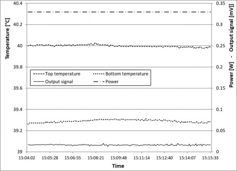
After ensuring the contact among the layers, with the conductive paste and a clamp, the heater was supplied with different input powers Qsup, reaching constant temperature values. Every test run about 30 minutes before stability condition, that was identified when their variation was under the sensors’ accuracy. In Figure 2 the main parameters are shown in time line for a typical stable test.
The steady-state condition was maintained for more than 10 minutes and, in this time interval, data were analysed and processed. During the overall campaign, the laboratory air temperature was around 24.8±1℃.
Figure 2. Main test parameters in stationary conditions
In Table 1, the average values are reported for the main parameters with absolute error underneath.
The RTD1 was used as reference condition and the electrical power was supplied to fix it from 35 to 65℃ with a 5 degrees step. The upper limit temperature of 90℃ was also achieved to test the rig stability and to verify the thermal conductivity variation in a wide span (out of the range of interest).
For every test the power was measured by a DC supply voltage V and current I (Eq. (1)):
Qsup =V⋅I (1)
Furthermore, the thermal loss was calculated through the polyurethane guard with Eq. (2) and the net power Qnet was derived in Eq. (3):
Qloss =AbkpΔxb(T1−T3)+AlkpΔxl(Tave −T4) (2)
Qnet=Qsup −Qloss (3)
where, Ab is the heater bottom surface, kp is the thermal conductivity of polyurethane (0.028 W/(m K) in this case), Δxb is the distance between RTD1 and RTD3 (20 mm), T1 and T3 are the temperature values, Al is the lateral surface of the internal block (made of aluminium layers, sample and heater), Δxl is the distance between the block and RTD4 (20 mm) with a measured value equal to T4 and Tave is the average of bottom and top temperatures (T1 and T2).
Once the net power through the sensitive element was derived, the thermal resistance of the internal block Rbl can be obtained setting out the expression provided by Eq. (4):
Qnet=T1−T2Rbl (4)
Rbl=Ral+Rcon +Rs (5)
Eq. (5) shows the different conductive contributions, respectively due to the aluminium layers Ral, contact paste Rcon and sample Rs. The first two counts for 0.0054 and 0.2439 K/W, respectively.
The third term contains the thermal conductivity ks of the sample that is the specific object of study (Eq. (6)):
Rs=ssAsks (6)
where, ss and As are the thickness and the contact surface of the component.
In the last column of Table 1, the calculated values of thermal conductivity are reported between 0.81 and 1.01 W/(m K).
Error evaluation was carried out considering all the contributes (type A and type B) as defined in the study [11]. Type A errors (σA) expressed the parameters stability during test, under constant boundary conditions, while Type B errors (σB) were related to the accuracy of used sensors and acquisition systems. They were summed in Eq. (7) to derive the overall precision (e) of direct measures such as temperatures, voltage, current:
e=√σ2A+σ2B (7)
For indirect measures, such as heating power, thermal loss, and thermal conductivity, the error propagation theory was applied considering the accuracy of single independent variables and the weight in the function that involves them.
Table 1. Test average parameters for thermal conductivity evaluation of the sensitive element
|
T1 [℃] |
T2 [℃] |
T1-T2 [℃] |
T3 [℃] |
T4 [℃] |
Tamb [℃] |
Qsup [mW] |
Qloss [mW] |
Qnet [mW] |
Vout [mV] |
ks [W/(m K)] |
|
|
1 |
35.0 |
34.3 |
0.7 |
25.5 |
25.2 |
23.8 |
320.0 |
80.6 |
239.4 |
14.57 |
1.01 |
|
±0.07 |
±0.07 |
±0.11 |
±0.07 |
±0.07 |
±0.07 |
±0.04 |
±0.6 |
±0.6 |
±0.03 |
±0.07 |
|
|
2 |
40.0 |
39.1 |
1.0 |
26.5 |
25.9 |
24.0 |
454.1 |
115.8 |
338.3 |
22.90 |
0.94 |
|
±0.08 |
±0.08 |
±0.11 |
±0.07 |
±0.07 |
±0.07 |
±0.04 |
±0.6 |
±0.6 |
±0.03 |
±0.05 |
|
|
3 |
45.0 |
43.8 |
1.2 |
29.7 |
28.9 |
26.5 |
503.0 |
131.4 |
371.6 |
27.59 |
0.86 |
|
±0.08 |
±0.08 |
±0.11 |
±0.07 |
±0.07 |
±0.07 |
±0.04 |
±0.6 |
±0.6 |
±0.05 |
±0.04 |
|
|
4 |
50.0 |
48.4 |
1.7 |
28.4 |
27.3 |
24.2 |
692.3 |
185.8 |
506.5 |
39.65 |
0.83 |
|
±0.08 |
±0.08 |
±0.12 |
±0.07 |
±0.07 |
±0.07 |
±0.04 |
±0.6 |
±0.6 |
±0.03 |
±0.03 |
|
|
5 |
55.0 |
53.0 |
2.0 |
29.5 |
28.4 |
24.6 |
832.0 |
218.0 |
614.0 |
47.65 |
0.85 |
|
±0.09 |
±0.09 |
±0.12 |
±0.07 |
±0.07 |
±0.07 |
±0.04 |
±0.6 |
±0.6 |
±0.04 |
±0.02 |
|
|
6 |
60.0 |
57.8 |
2.2 |
32.1 |
30.7 |
26.4 |
945.4 |
239.5 |
705.9 |
54.58 |
0.85 |
|
±0.09 |
±0.09 |
±0.12 |
±0.07 |
±0.07 |
±0.07 |
±0.04 |
±0.7 |
±0.7 |
±0.04 |
±0.02 |
|
|
7 |
65.0 |
62.4 |
2.6 |
31.6 |
29.8 |
24.9 |
1075.9 |
287.2 |
788.7 |
64.67 |
0.81 |
|
±0.09 |
±0.09 |
±0.13 |
±0.07 |
±0.07 |
±0.07 |
±0.04 |
±0.7 |
±0.7 |
±0.04 |
±0.02 |
|
|
8 |
90.0 |
85.5 |
4.5 |
36.5 |
33.3 |
24.6 |
1854.4 |
461.7 |
1392.7 |
109.50 |
0.84 |
|
±0.11 |
±0.11 |
±0.2 |
±0.07 |
±0.08 |
±0.07 |
±0.06 |
±0.7 |
±0.7 |
±0.06 |
±0.01 |
It is important to note that temperature difference (T1 - T2) was always under 2℃ for test 1-2-3-4 and the relative total uncertainty overcome 7%. This fact gets close combined uncertainty for conductivity over 3% in the same range. In particular, the combined uncertainty enabled the calculation of each investigated parameter as a function of other parameters directly measured with known error.
For this reason, only the Test 5-6-7-8 were considered for the average value of ks evaluation, which resulted 0.84±0.01 W/(m K).
The conductivity had the same value for test 8 at 90℃. This fact suggested a negligible variation in a wide range of temperature.
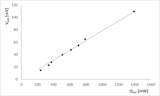
During test, the output voltage from the sensitive element was monitored and summarised in Table 1 as Vout [mV]. The trend in relation to net power is linear with a good approximation as shown in Table 2 and Figure 3, imposing the passage from zero.
It is important to notice that, at each reported study phase, the thermal power flux was always above 100 W/m2.
Table 2. Linear regression and statistical parameters for the output signal to thermal power function
|
Linear coefficient |
Standard error |
Constant term |
R2 |
|
0.078 |
0.001 |
0 |
0.998 |
Figure 3. Output signal of the sensitive element as a function of the net power passing through
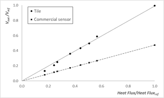
Figure 4. Calibration curves of Tile in comparison with a commercial sensor
This value exceeded decisively the one expected for building sector (few tens of W/m2). Anyway, the imposed settings were necessary to ensure suitable accuracy conditions during test, especially related to the measurement of temperature difference across the sensitive element. This fact allowed to derive the thermal conductivity of the component and to demonstrate the capability of its application. We believe that more specific analyses should be developed and addressed to signal quality investigation.
The sensitive element potential for measurement scopes, the obtained calibration curve was compared with the corresponding curve of a common commercial sensor (Figure 4). According to the data sheet, the Tile output signal for each heat flux value, inside the range of interest, resulted twice the amount of the others.
2.2 The frame design for the heat flux sensor
In the previous section, the investigation on the component made of semi-conductor junctions, showed its thermal and electrical properties and suggested the application for heat flux measurement on building systems. A complete sensor was properly designed and realised as a prototype.
The first main task was to extend the measuring reference surface beyond the dimensions of the sensitive component. A specific frame was set up, exceeding the issues suggested by Trethowen [21], with a reduction of the global “edge to surface area” which amounted to 0.4 at the beginning.
One fundamental constrain was fixed for ensuring the consistency of the measurement: the sensor stratigraphy was kept at homogenous thermal properties (global resistance) in the section where the sensitive element is present and around it. Only in this condition, the same measured heat flux can be properly addressed on the overall sensor surface, without significant distortions. Aluminium plates were chosen as external edge surfaces to avoid transversal temperature gradient, due to its high conductivity.
Different materials were investigated to design the frame. A scheme of the obtained layout is shown in Figure 5 (the picture dimensions are not in scale to give a better comprehension). It is composed by the external aluminium plates, 1 mm layer of lexan polycarbonate and 3 mm graphite layer. The aluminium plates are notched 40x40 mm2 for 0.3 mm in the centre, to place the sensitive element with a thin silicon filler: this choice guarantees the contact and the conductive heat transfer process without air gaps.
Each layer was identified on the base of thermal conductivity kl and thickness sl, corresponding to the specific material, aiming at a global resistance value Rl (per unit area) as close as possible to the resistance in the section where the sensitive element was placed. Table 3 shows the main parameters for the sensor stratigraphy. The difference between the two thermal resistances was found under 2%.
Figure 5. Transversal section of a sensor with different layers and sensitive element in the centre
Table 3. Sensor stratigraphy
|
Stratigraphy with sensitive element |
Stratigraphy around sensitive element |
||||||
|
kl [W/(m K)] |
sl [mm] |
Rl [K/W] |
kl [W/(m K)] |
sl [mm] |
Rl [K/W] |
|
|
|
Aluminum |
230 |
1.7 |
7.39 10-6 |
230 |
2 |
8.70 10-6 |
Aluminum |
|
Contact interface |
1.3 |
0.3 |
2.31 10-4 |
25 |
3 |
1.20 10-4 |
Graphite |
|
Sensitive element |
0.84 |
4 |
4.76 10-3 |
0.2 |
1 |
5.00 10-3 |
Lexan Polycarbonate |
|
Contact filler |
1.3 |
0.3 |
2.31 10-4 |
230 |
2 |
8.70 10-6 |
Aluminum |
|
Aluminum |
230 |
2.7 |
7.39 10-6 |
|
|
|
|
|
Tot. |
8 |
5.24 10-3 |
|
8 |
5.14 10-3 |
|
|
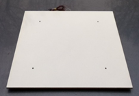
The sensor, called Tile, was made up in some prototypes, painting with white colour the external surface, to limit the heat exchange due to thermal radiative phenomena (Figure 6). Another paint (taken from automotive sector) was used to paste the different components each other, by a spray machine. The glue was not considered in the global thermal resistance evaluation, because the thickness of the adhesive layer was taken less than 0.1 mm. A maximum dimension of 530x530 mm2 was chosen for manufacturing feasibility, reducing the “edge to surface area” value from 0.4 to 0.06 [21].
Important effects of the specific sensor in situ application and the expected deflection in measured values of the heat flux through the walls of a building, were investigated. Cocumo et al. [26] has proposed a procedure to evaluate the HFS influence, combining its properties and wall characteristics. In this case, the sensor is placed on the internal wall (that is the most probable configuration) the ratio between the one-dimensional flux Qs0due to the HFS presence and the undisturbed flux Q0 is expressed by Eq. (8):
Qs0Q0=(Rci+RwRci+Rw+Rs) (8)
where, Rci is the internal convective/radiative contribute due to global thermal resistance (no sun light advised), Rw is the wall resistance, and Rs the resistance of sensor. Considering a real case study for the HFS application, the parameter values were assumed as follows:
With these constrains, the ratio between the heat flux with and without the sensor is very close to 1 and the deviation induced by the HFS is under 1‰.
The same order of magnitude is reached if the convective/radiative contribute is halved and the wall resistance is doubled (the worst condition). On this matter, the large guard ring (sensor width more than 4 times of the sensitive element width) produced a good effect.
Figure 6. The sensor Tile
The laboratory test of materials and solutions for building application is a standard procedure described by EN 12664: 2001. They are fundamental for the thermal characterization and comparison at the same controlled repeatable constrains. In situ measurements are also necessary in order to verify the response at real dynamic conditions during their lifetime. Moreover, the influence of the human behaviour has to be addressed since the operative regimes are strongly modified by way of life and different use and activities in indoor environments. A new heat flux sensor development was shown and discussed, from the preliminary design to prototype realization.
The research started from a low-cost commercial component, which was supposed to be proper for the application as a sensitive element. After the characterization of its thermal conductivity under hot guard plate test (0.84±0.01 W/(m K)), some improvements were proposed designing a specific frame with similar thermal resistance (0.00514 K/W) in order to let the measurement more reliable. This could be achieved by using two layers of different materials (e.g. graphite and lexan polycarbonate).
As mention before, the aluminum plates were added in order to homogenize surface temperatures and also to guarantee the suitable stiffness.
ISO 9869:2014 [11] indicates the ranges of the main HFS parameters that are reported in Table 4 with the values related to Tile sensor on the right. It is shown that they are within the limits, except for the overall thickness that exceed of 3 mm. It is to say that, after the realization of prototype, the structure appears enough rigid suggesting the aluminum plates could be reduced: this task is under investigation.
The analysis on the expected thermal resistance of sensor referred to typical wall properties let to verify the alteration in the heat flux in the proximity of measurement set-up.
Table 4. Suggestions for HFS by ISO 9869:2014
|
Parameter |
Range |
Tile values |
|
Diameter of the active part |
10-500 mm |
40x40 mm |
|
Total diameter of the HFS |
10-600 mm |
530x530 mm |
|
Thickness of the facings |
0.1-5 mm |
2 mm |
|
Th. conductivity of the facings |
0.03-400 W/(m K) |
230 W/(m K) |
|
Th. conductivity of the passive part |
0.03-2 W/(m k) |
0.84 W/(m K) |
|
Th. resistance of active part |
0.001-0.01 K/W |
0.00524 K/W |
|
Thickness of the sensor |
0.2-5 mm |
8 mm |
The new HFS is resulted not intrusive such as it does not affect the measurement substantially (less than 1‰). At last, the study demonstrated that sensor has the suitable thermal properties for the application in building context. A proper calibration is needed to verify the relation between the output signal and the heat flux. The preliminary analysis presented at the end of par. 2.1 showed it is linear in a wide range. Another important result is that the expected output values are in the order of mvolt even for a heat flux under 20 W/m2. It represents a very promising feature for a passive sensor in order to obtain more reliable measurements.
The authors thank all those engineering students that cooperated during the experimental test and data post-processing.
|
RTD |
Resistance Temperature Detector |
|
Qsup |
Thermal power supplied during test due to the Joule effect [W] |
|
V |
DC Voltage supplied during test [V] |
|
I |
DC current supplied during test [A] |
|
Qloss |
Thermal power loss around the test rig [W] |
|
Qnet |
Net thermal power across the sample during test [W] |
|
kl |
Thermal conductivity of the layer [W/(m K)] |
|
sl |
Thickness of the layer [mm] |
|
Ab |
Heater bottom area [m2] |
|
kp |
Thermal conductivity of insulation [W/(m K)] |
|
Δxb |
Distance between temperature sensors through the insulation under the heater [m] |
|
Al |
Lateral area of the block with the sensitive element [m2] |
|
Δxl |
Distance between temperature sensors through the insulation next to the sample [m] |
|
T1 |
Temperature under the sample [°C] |
|
T2 |
Temperature above the sample [°C] |
|
T3 |
Temperature in the insulation under the heater [°C] |
|
T4 |
Temperature in the insulation next to the sample [°C] |
|
Tave |
average between T1 and T2 [°C] |
|
Rl |
Thermal resistance of the layer [K/W] |
|
Rbl |
Global thermal resistance of the internal block of the rig [K/W] |
|
Ral |
Aluminium plate thermal resistance [K/W] |
|
Rcon |
Contact paste thermal resistance [K/W] |
|
Rs |
Sample thermal resistance [K/W] |
|
As |
Sample bottom area [m2] |
|
ks |
Sample thermal conductivity [W/(m K)] |
|
ss |
Sample thickness [m] |
|
Tamb |
Laboratory air temperature [°C] |
|
Vout |
Sample output signal [mV] |
|
Q0 |
Undisturbed Heat flux through a wall [W/m2] |
|
Qs0 |
Heat flux through a wall with HFS [W/m2] |
|
Rci |
Convective and radiative contribution to thermal resistance [K/W] |
|
Rw |
Thermal resistance of wall [K/W] |
|
e |
Total error for direct measures |
|
σA |
Type A error |
|
σB |
Type B error |
[1] European Commission. Green Paper: A 2030 climate & energy framework, COM (2013). 169. https://ec.europa.eu/clima/policies/strategies/2030_en, accessed on 12 June 2020.
[2] European Parliament. Directive 2010/31/eu, May 2010. https://ec.europa.eu/energy/topics/energy-efficiency/energy-efficient-buildings/energy-performance-buildings-directive_en, accessed on 12 June 2020.
[3] Distefano, D.L., Gagliano, A., Naboni, E., Sapienza, V., Timpanaro, N. (2018). Thermophysical characterization of a cardboard emergency kit-house. Mathematical Modelling of Engineering Problems, 5(3): 168-174. https://doi.org/10.18280/mmep.050306
[4] Baccilieri, F., Bornino, R., Fotia, A., Marino, C., Nucara, A., Pietrafesa, M. (2016). Experimental measurements of the thermal conductivity of insulant elements made of natural materials: Preliminary results. International Journal of Heat and Technology, 34(S2): S413-S419. https://doi.org/10.18280/ijht.34S231
[5] Cardinale, T., Arleo, G., Bernardo, F., Feo, A., De Fazio, P. (2017). Investigations on thermal and mechanical properties of cement mortar with reed and straw fibers. International Journal of Heat and Technology, 35(S1): S375-S382. https://doi.org/10.18280/ijht.35Sp0151
[6] Cardinale, T., Sposato, C., Alba, M.B., Feo, A., Grandizio, F., Lista, G.F., Montesano, G., De Fazio, P. (2019). Energy and mechanical characterization of composite materials for building with recycled PVC. Italian Journal of Engineering Science, 63: S129-135. https://doi.org/10.18280/ti-ijes.632-403
[7] Amara, I., Mazioud, A., Boulaoued, I., Mhimid, A. (2017). Experimental study on thermal properties of bio-composite (gypsum plaster reinforced with palm tree fibers) for building insulations. International Journal of Heat and Technology, 35(3): 576-584. https://doi.org/10.18280/ijht.350314
[8] Boudenne, A., Ibos, L., Gehin, E., Candau, Y. (2004). A simultaneous characterisation of thermal conductivity and diffusivity of polymer materials by a periodic method. Journal of Physics D: Applied Physics, 37(1): 132-139. https://doi.org/10.1088/0022-3727/37/1/022
[9] Cesaratto, G., De Carli, M. (2013). A measuring campaign of thermal conductance in situ and possible impacts on net energy demand in buildings. Energy and Buildings, 59: 29-36. http://dx.doi.org/10.1016/j.enbuild.2012.08.036
[10] Biddulph, P., Gori, V., Elwell, C.A., Scott, C., Rye, C., Lowe, R., Oreszczyn, T. (2014). Inferring the thermal resistance and effective thermal mass of a wall using frequent temperature and heat flux measurements. Energy and Buildings, 78: 10-16. http://dx.doi.org/10.1016/j.enbuild.2014.04.004
[11] ISO 9869-1:2014, Thermal Insulation - Building Elements - In-Situ Measurements of Thermal Resistance and Thermal Transmittance. International Organization for Standardization, Geneva.
[12] Diller, T. (1993). Advanced in Heat Transfer. Academic Press. 1-471.
[13] Childs, P.R.N., Greenwood, J.R., Long, C.A. (1999). Heat flux measurement techniques. Journal of Mechanical Engineering Science, 213(7): 655-677. https://doi.org/10.1177/095440629921300702
[14] Flanders, F.N. (1999). Heat flux transducers measure in-situ building thermal performance. Journal of Thermal Insulation and Building Envelopes, 18(1): 28-52. https://doi.org/10.1177/109719639401800103
[15] Degenne, M., Klarsfeld, S. (1985). A new type of heat flowmeter for application and study of insulation and systems. Building Applications of Heat Flux Transducers, 163-171. https://doi.org/10.1520/STP32936S
[16] Langley, L.W., Barnes, A., Matijasevic, G., Gandhi, P. (1999). High-sensitivity, surface-attached heat flux sensors. Microelectronics Journal, 30(11): 1163-1168. http://dx.doi.org/10.1016/S0026-2692(99)00080-4
[17] Zhang, C., Huang, J., Li, J., Yang, S., Ding, G., Dong, W. (2019). Design, fabrication and characterization of high temperature thin film heat flux sensors. Microelectronic Engineering, 217: 111128. https://doi.org/10.1016/j.mee.2019.111128
[18] Gidik, H., Bedek, G., Dupont, D., Codau, C. (2015). Impact of the textile substrate on the heat transfer of a textile heat flux sensor. Sensors and Actuators A: Physical, 230: 25-32. http://dx.doi.org/10.1016/j.sna.2015.04.001
[19] Clayton, C.A., Diller, T.E. (2010). In situ high temperature heat flux sensor calibration. International Journal of Heat and Mass Transfer, 53(17-18): 3429-3438. https://doi.org/10.1016/j.ijheatmasstransfer.2010.03.042
[20] Saidi, A, Kim, J. (2004). Heat flux sensor with minimal impact on boundary conditions. Experimental Thermal and Fluid Science, 28(8): 903-908. https://doi.org/10.1016/j.expthermflusci.2004.01.004
[21] Trethowen, H. (1986). Measurement errors with surface-mounted heat flux sensors. Building and Environment, 21(1): 41-56. https://doi.org/10.1016/0360-1323(86)90007-7
[22] ISO 8302:1991, Thermal Insulation - Determination of Steady-State Areal Thermal Resistance and Related Properties - Guarded Hot Plate Apparatus, International Organization for Standardization.
[23] ASTM C 177. (2019). Standard Test Method for Steady-State Heat Flux Measurements and Thermal Transmission Properties by Means of the Guarded Hot Plate Apparatus, Annual Book of ASTM Standards. https://doi.org/10.1520/C0177-19
[24] ASTM C 518. (2017). Standard Test Method for Steady-State Thermal Transmission Properties by Means of the Heat Flow Meter Apparatus, Annual Book of ASTM Standards. https://doi.org/ 10.1520/C0518-17
[25] Cocumo, M., Ferraro, V., Kaliakatsos, D., Mele, M. (2018). On the distortion of thermal flux and of surface temperature induced by heat flux sensors positioned on the inner surface of buildings. Energy and Buildings, 158: 677-683. https://doi.org/10.1016/j.enbuild.2017.10.034