Anwer F. Faraj | Itimad D.J. Azzawi* | Samir G. Yahya
© 2020 IIETA. This article is published by IIETA and is licensed under the CC BY 4.0 license (http://creativecommons.org/licenses/by/4.0/).
OPEN ACCESS
A computational fluid dynamics (CFD) study was conducted to analyse the flow structure and the effect of varying the coil pitch on the coil friction factor and wall shear stress, through utilising different models’ configurations. Three coils were tested, all of them having the same diameter and coil diameter: 0.005m and 0.04m respectively. Pitch variations began with 0.01, 0.05, 0.25 m for the first, second and third model respectively. Two turbulence models, STD(k-ϵ) and STD(k-w), were utilised in this simulation in order to determine the turbulence model which could capture most of the flow characteristics. A comparison was made between the STD(k-ϵ) and STD(k-w) models in order to analyse the pros and cons of each model. The results were validated with Ito’s equation for turbulent flow and compared with Filonenko’s equation for a straight pipe. The governing equations were discretized using finite volumes method and the SIMPLE algorithm was used to solve the equations iteratively. All the models were simulated using the ANSYS Fluent solver CFD commercial code. The results showed that in turbulent flows, Dean number had a stronger effect on reducing coil friction factor than the increment in pitch dimension.
CFD, helical coil, friction factor, Reynolds number, pitch size, turbulent flows
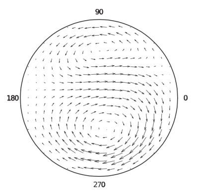
Flows following a curved path induce a centrifugal force which pushes the faster fluid particles outwards, whereas the slower ones are pushed inwards; and since the centrifugal force depends on the local axial velocity, therefore the slower particles suffer a lower centrifugal effect while the faster ones experience higher centrifugal forces [1]. The existence of the boundary layer determines the effect of the centrifugal force, where the fluid particles near the wall undergo a small effect while the fluid particles in the core of the pipe experience the opposite effect. The imbalance in the centrifugal forces develops a secondary flow which ends with two-counter rotating vortices called Dean Vortices as shown in Figure 1 [2]. The secondary flow, in turn, increases flow mixing which consequently increases the rate of heat transfer in comparison with a straight pipe.
Figure 1. Dean vortices [3]
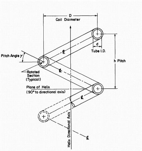
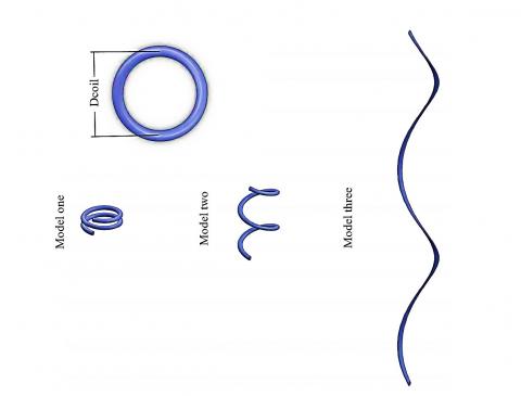
Dean vortices are named after the British scientist Dean [4]. Dean vortices, which are generated from the unsteadiness of the centrifugal forces, appear in many engineering applications such as turbine blades and cooling passages inside engines. The secondary flow intensity increases as the curvature increases. Dean vortices cause an important modification to the boundary-layer structure which leads to a greater enhancement in the rate of heat transfer. Furthermore, these vortices have an effect in delaying the transition from laminar to turbulent flow [5]. Moreover, the controlling parameters in helically coiled pipes are curvature ratio ($\delta$), Reynolds number ($R_{e}$), Dean Number ($D_{e}$), Torsion parameter ($\beta_{0}$) and pitch size and the calculating formula for each parameter is available by Austen and Soliman [6] and not repeated here. Figure 2 defines these parameters especially the distance between the centerline of two turns.
Figure 2. The parametric explanation of helically coiled pipe [6]
The following section presents an outline of selected research papers investigating turbulent flows in helically coiled pipe. Experimental and numerical (using CFD) techniques will be studied and analysed for different parameters which have a direct effect on the secondary flow formulation. These parameters are Dean Number, curvature ratio, pitch size and pipe diameter, and the effect of these parameters on the rate of heat transfer. In this section, attention will be paid to the flow structure particularly in a fully developed region in terms of pressure drop, pitch size, and curvature ratio, which plays a leading role in determination of wall shear stress and consequently the coil friction factor at turbulent flow. Moreover, different turbulent models will be assessed in terms of accuracy in capturing the secondary flow phenomena and stability of the solution.
Hüttl and Friedrich [7] studied the turbulent fully developed flow in curved and helically coiled pipes but using a different simulation scheme from that used by Yamamoto et al. [8] and Hüttl and Friedrich [9]. A direct numerical simulation with a specific Reynolds number $R e_{\tau}=230$ was used by Hüttl and Friedrich [9]. It was stated that for a great value of curvature parameter ($k=0.1$), the turbulence is reduced by the streamwise curvature and the flow is approximately relaminarised [7]. The torsion has a relatively small effect in this region in comparison with the curvature effect. However, it cannot be negligible. The dissipation rate and the fluctuations of turbulent kinetic energy are increased since the torsion has an influence on the secondary flow which has been activated by a curvature.
Although laminar and turbulent flows in straight pipes have been widely investigated, turbulent flows in helically coiled pipes still need to be examined and their flow structure studied. In fact, that motivated Hüttl and Friedrich [9] to use Direct numerical simulation to demonstrate the similitudes and contrasts between the flows in curved and helical pipes. It has been concluded that the turbulent fluctuations in straight pipes are much larger than their counterparts in a curved pipe. Furthermore, the comparison between the mean axial velocity in a helical and toroidal pipe shows relatively small differences. The torsional effect is extremely small compared to the curvature ratio effect. However, it cannot be ignored, due to the fact that the torsion is responsible for inducing the secondary flow and consequently, the turbulent kinetic energy is increased by Hüttl and Friedrich [9]. A comparison also between many turbulence models with completely resolved direct numerical simulation, at $y^{+}=1.2$ i.e. inside the viscous affected region with a specific characteristic of Reynolds number and the curvature ratio was investigated by Castiglia et al. [10] and in this research the curvature ratio has been taken as a constant. It has been found that Reynolds number and the curvature ratio are the most critical factors for the turbulence flow.
Although $(k-\epsilon)$ model is extensively used in many types of flow and presents a quite acceptable result, the $(k-\epsilon)$ model, even with special near wall treatment, failed to correctly predict the behaviour of the Darcy-Weisbach friction coefficient. To overcome the shortcomings of the above DNS results, SST and RSM have been used to obtain an adequate agreement with the experimental data, particularly at low Reynolds numbers. The first investigation which concerns the development of turbulent forced convection heat transfer in helical pipes was done by Lin and Ebadian [11]. This investigation covered a wide range of influential parameters as listed below:
The numerical result shows a good agreement with the experimental data [12], as shown in Figure 3 below.
Figure 3. Nusselt number validation with experimental results for non-dimensional pitch=0 [11]
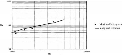
A numerical study using the $(k-\epsilon)$ model is available [13], but with a large pitch. This study was validated with other experimental data of Mori and Nakayawa [14], with satisfactory results as shown in Figure 4 below.
Figure 4. Comparison of the numerical results with the experimental findings [13]
Moreover, Rogers and Mayhew [12] conducted an experiment mainly to check out the surface roughness of the pipe, in order to do that the pressure losses are significantly hypersensitive in comparison with the heat transfer information. They have used Eq. (1), in order to determine the overall heat transfer coefficient (U).
$Q=U \log {mean} \Delta t$ (1)
where, $\Delta t=\frac{\left(t_{g}-t_{b 1}\right)-\left(t_{g}-t_{b 2}\right)}{\operatorname{Ln} \frac{\left(t_{g}-t_{b 1}\right)}{\left(\operatorname{tg}-t_{b 2}\right)}}$.
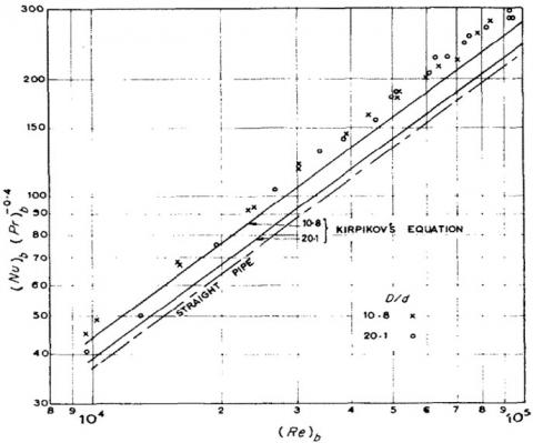
A comparison has been made with Kirpikov’s [15] findings with different curvature ratios to calculate the heat transfer rate. In Figure 5, it can be seen that using Kirpikov's relationship shown in Eq. (2), to denote the y-axis in Figure 5, with different curvature ratio does not make a large difference in terms of heat transfer rate as clearly seen in Figure 5.
$Q=U \log {mean} \Delta t$ (2)
It was found that the results of Rogers and Mayhew [12] are 10% more than Kirpikov’s findings and 10% less than those obtained by Seban and McLaughlin’s [16] experiment. It is suggested that more work is needed to determine the exact exponent value of $\left(\frac{d}{D}\right)$.
Figure 5. Heat transfer findings, properties evaluated at bulk temperature [12]
Bai et al. [17] did an experiment to find the most appropriate correlation for measuring the average heat transfer coefficient at different cross-sections of helically coiled pipe. Although many investigations have been done previously by Rogers et al. [12, 14-16], it was still necessary to establish a correlation which would cover a wide range of horizontal helically coiled pipes and to gain more profound comprehension of the local heat transfer attributes in both axially and circumferential directions.
$\frac{N u_{L}}{N u}=0.22\left(\frac{R_{e} P_{r}}{10^{4}}\right)^{0.45}\left(0.5+0.1 \theta+0.2 \theta^{2}\right)$ for $0<$$\theta \leq \pi$ (3)
Three models of horizontally-oriented helically coiled pipe have been utilised with two turns, to ensure that flow reaches a fully developed region [18], and different pitches as shown in Figure 6. The pipe and coil diameters are taken respectively as d=0.005m, Dcoil=0.04m with different pitches P= (0.01, 0.05, and 0.25) m as shown in Table 1.
Figure 6. Models geometry plotted in 2:1 scale
Table 1. Models dimensions
|
Models |
Pipe diameter (d) m |
Coil diameter (Dcoil) m |
Pitch (P) m |
|
Model one |
0.005 |
0.04 |
0.01 |
|
Model two |
0.005 |
0.04 |
0.05 |
|
Model three |
0.005 |
0.04 |
0.25 |
In Table 1, the pipe and coil diameters are constants, but the pitch is different. The second and third models are designed to explore the effect of a varying pitch on the secondary flow structure. The two vortices are symmetrical if the pipe is bent in a toroidal shape, but if the bent in a helically shape the symmetry breaks up [1]. Stretching helically coiled pipe while keeping the pipe and coil diameter constant needs an increment in the helix length. The helix length of the three models has been calculated with a very simple basic equation derived from Pythagoras-theorem as shown in Eq. (4) bellow:
$helix\, length=\left[( { Coil\, circumference })^{2}+\right.$$\left.( { Pitch })^{2}\right]^{1 / 2} \times N$ (4)
where, N= number of turns.
Moreover, two surfaces were defined in the geometry in a fully developed region: specifically, in the last quarter of the helically coiled pipe before the outlet, as shown in Figure 7. Plane two is located well downstream of the inlet to guarantee fully developed flow conditions; one coil turn is enough to assure fully developed flow [18], while plane one is located near the outlet, to avoid the processed arrangement of being influenced by the outlet boundary conditions. The purpose of these two planes is to evaluate the average pressure at each plane, then compute the pressure difference in order to obtain the wall shear stress in a fully developed area.
Figure 7. Positions of planes for P=0.05m
2.1 Computational domain and solution procedure
A comparison has been made between the one-domain automatic generated and five-domain O-H grid method “butterfly topology” mesh as shown in Figures 8-a to 8-c. It has been found that ordinary automatic generated mesh has considerable skewness particularly near the wall, which is considered an important region, especially when studying the near wall behaviour (Figure 8-a). In Figures 8-b, when the five-domain O-H grid method “butterfly topology” mesh is applied, greater reduction in the maximum included angle is obtained i.e. the maximum included angle is reduced from 175.35° to 130.2°, which helps to increase the stability and accuracy of the solution. After selecting Grid-solver and running the solver, the maximum included angle is decreased again to 124.8° and most of the cells become orthogonal. The percentage of cells with an angle of 121°-124° does not exceed 10% of the total cells, as shown in Figures 8-c, and this mesh may be considered the best mesh which can capture most of the flow characteristics.
Figure 8. The one (a) to five (c) domain automatic generated mesh with the maximum included angle
In order to obtain a grid independent solution, different simulations were run with different mesh arrangements. Four cases of mesh: coarse (95,956 cells), medium (185,623cells), fine (313,823cells) and very fine mesh (597,600 cells), as shown in Figure 9 (see Table 2 for further details), were studied and analysed to choose an adequate mesh which gives acceptable results with minimum errors and computer resources in addition to a satisfactory computational time.
Table 2 showed that the mesh has been used with different numbers of cells to acquire a mesh independent solution. It can be seen that there is no great difference in maximum velocity in all types of mesh i.e. all of them have the same difference of 0.001. However, the difference between the very fine mesh and the course is 0.003. In order to attain the most appropriate mesh which can capture most of the flow characteristics, one may need to choose the mesh where there is no difference in results as the mesh size is increased. The fine mesh gives satisfactory results in addition to saving computational time and reducing the requirement for computer resources because of the large difference in cell numbers between the fine and very fine mesh, which leads to a small difference in the findings. For the above reasons, the fine mesh has been chosen to simulate the three models. Moreover, the mesh study using the maximum velocity has been validated by using the values of CFD Fanning friction factor with different cell numbers. It has been found that the difference in CFD Fanning friction factor between the fine and very fine mesh is quite low (0.0004), which makes it unnecessary to increase the mesh size if the difference is ignorable. Hence, the fine mesh has been chosen in the simulation.
Figure 9. Mesh Generation from coarse to very fine mesh
Table 2. Different mesh arrangements with their number of cells, maximum velocity and friction factor
|
Mesh type |
Total mesh |
Maximum velocity |
Friction factor |
|
Coarse mesh |
95,956 |
0.174 |
0.053393 |
|
Medium mesh |
185,623 |
0.175 |
0.064598 |
|
Fine mesh |
313,823 |
0.176 |
0.065634 |
|
Very fine mesh |
597,600 |
0.177 |
0.065196 |
The governing equations applied to the models to calculate the friction factor and wall shear stress are available in the studies [1, 19] and not repeated here. However, in a fully developed region, i.e. when the velocity gradient is constant, the wall shear stress can be computed from the static pressure drop over a determined length of pipe [1]. There are many experimental equations which can be used to predict the friction factor and the pressure in a helically coiled pipe, for instance: [2, 14, 20-25]. All of these present an acceptable agreement between their correlations, since Ali [18] has made a comparison between the aforementioned correlations which gave almost convergent results.
Ito’s equations have been adopted in the calculations because they are practical and easy to implement. Furthermore, this is the most accurate formula [10]. On the other hand, White’s equations do not work with the model’s dimensions since they are limited to De<11.6 and Re<100,000. Mori equation is complicated while Misra and Gupta's equations used what is called (He) helical number which made the equations drastically complicated and limited. For the above reasons, Ito’s equations have been chosen to compute the coil friction factor.
The boundary conditions for the helically coiled pipe simulation were set as water domain fluid with turbulent flow velocity inlet condition. Three Reynolds numbers (15000, 50000 and 100000) were used in the simulation i.e. different velocity values were set at the inlet for each pitch to examine the flow structure as the pitch changed. Moreover, the wall is taken as a stationary wall and no-slip condition is applied to the wall, while the outlet is taken as a pressure outlet.
Pressure based solver was chosen for the helically coiled pipe simulation since it is generally used for the incompressible fluid. The SIMPLE [Semi-Implicit Method for Pressure-Linked Equations] algorithm by Patankar and Spalding [26] was used in order to discretise the velocity field through the solution of the momentum equation. The Green-Gauss cell-based theorem was set to evaluate the scalars at the cell centroid. The second order upwind scheme was used for momentum, turbulent kinetic energy, specific dissipation rate and turbulent dissipation rate.
4.1 Turbulent model
The $(k-\epsilon)$ model was the most usable model until the last decade of the 20th century. It had been developed by Chou et al. [27-29]. This model started to be used widely when the updated version of the $(k-\epsilon)$ model had been presented by Jones and Launder [30]. The model was then modified again by Launder and Sharma [31] and became what is generally called the STD $(k-\epsilon)$ model [32].
The STD $(k-\epsilon)$ model’s equations are listed below [32]:
Kinematic eddy viscosity:
$v_{T}=C_{\mu} \frac{k^{2}}{\epsilon}$ (5)
Turbulent kinetic energy:
$\frac{\partial k}{\partial t}+U_{j} \frac{\partial k}{\partial x_{j}}=\tau_{i j} \frac{\partial U_{i}}{\partial x_{j}}-\epsilon+\frac{\partial}{\partial x_{j}}\left[\left(v+\frac{v_{T}}{\sigma_{k}}\right) \frac{\partial k}{\partial x_{j}}\right]$ (6)
Dissipation rate:
$\frac{\partial \epsilon}{\partial t}+U_{j} \frac{\partial \epsilon}{\partial x_{j}}=C_{\epsilon 1} \frac{\epsilon}{k} \tau_{i j} \frac{\partial U_{i}}{\partial x_{j}}-C_{\epsilon 2} \frac{\epsilon^{2}}{k}+\frac{\partial}{\partial x_{j}}[(v+$$\left.\left.\frac{v_{T}}{\sigma_{\epsilon}}\right) \frac{\partial \epsilon}{\partial x_{j}}\right]$ (7)
Launder et al. [33] have recommended after wide research of free turbulent flows that the constants appearing in Eqns. (5), (6) and (7) can be tabulated as shown in Table 3 below:
Table 3. Constants in the STD $(k-\epsilon)$ model
|
$C_{\epsilon 1}$ |
$C_{\epsilon 2}$ |
$\boldsymbol{\sigma}_{\boldsymbol{k}}$ |
$\boldsymbol{\sigma}_{\boldsymbol{\epsilon}}$ |
$\boldsymbol{c \mu}$ |
|
1.44 |
1.92 |
1.0 |
1.3 |
0.09 |
These equations are connected together by the length scale as shown in Eq. (8) which is easy to describe [34]:
$l=C_{\mu} \frac{k^{3 / 2}}{\epsilon}$ (8)
The STD $(k-w)$ model in ANSYS Fluent is formulated on Wilcox model [32]. The first equation is for the turbulent kinetic energy while the second equation is for the specific dissipation rate (w), where:
$w=\frac{\epsilon}{\left(\beta^{*} k\right)}$ (9)
The equations of the $(k-w)$ model is listed below:
Eddy viscosity:
$v_{T}=\frac{k}{w}$ (10)
Turbulence kinetic energy:
$\frac{\partial k}{\partial t}+U_{j} \frac{\partial k}{\partial x_{j}}=\tau_{i j} \frac{\partial U_{i}}{\partial x_{j}}-\beta^{*} k w+\frac{\partial}{\partial x_{j}}\left[\left(v+\sigma^{*} v_{T}\right) \frac{\partial k}{\partial x_{j}}\right]$ (11)
Specific dissipation rate:
$\frac{\partial w}{\partial t}+U_{j} \frac{\partial w}{\partial x_{j}}=\alpha \frac{w}{k} \tau_{i j} \frac{\partial U_{i}}{\partial x_{j}}-\beta w^{2}+\frac{\partial}{\partial x_{j}}[(v+$$\left.\left.\sigma v_{T}\right) \frac{\partial w}{\partial x_{j}}\right]$ (12)
Closure coefficients and auxiliary relations:
$\alpha=\frac{5}{9}, \beta=\frac{3}{40}, \beta^{*}=0.09, \sigma=0.5, \sigma^{*}=0.5$ (13)
The dissipation and the specific dissipation rate are connected together by the following equation:
$\epsilon=\beta^{*} w k$ (14)
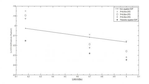
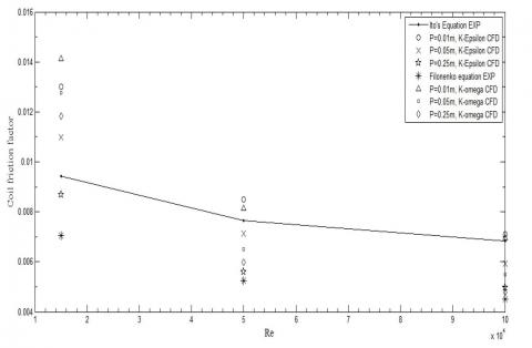
A comparison has been made between Ito’s experimental equation for the turbulent flows and the CFD simulation results of the three models as shown in Figure 10. In terms of the straight pipe, it can be seen that Filonenko’s equation [19], has been used instead of Colebrook's [34] equation for the turbulent flow. The reason is that the Fanning friction factor correlation with the Reynolds number is quite complicated and it is controlled by Colebrook’s equation below.
$\frac{1}{\sqrt{f}}=-4.0 \log _{10}\left[\frac{\frac{\gamma}{d}}{3.7}+\frac{1.256}{R_{e} \sqrt{f}}\right]$ (15)
In terms of the coil friction factor of P=0.01m, it can be seen that the discrepancy between the experimental result of Ito’s equation and the CFD coil friction factor decreases as the Reynolds number is increased and the overall trend is quite satisfactory. particularly at Re=15,000, is that this might be wrong because of the big difference between the experimental and the CFD result, but in fact, the difference does not exceed 0.5% which is good; while for the other Reynolds numbers the difference is much less, around 0.05% which is excellent. These results reflect the reasons behind considering the STD $(k-\epsilon)$ model as the workhorse of the most frequently encountered flow engineering applications in the industry in spite of its limitations and shortcomings (for example, numerical stiffness and poor performance in complex flow that contains steep curvature and strong pressure gradient), since it is robust and computationally cheap [35].
Turning to discuss the results of the second model (P=0.05m), when Re=15,000, the coil friction factor value is higher than Ito’s equation, but it less than its equivalent for P=0.01m. However, the difference between the coil friction factor values of P=0.01m and P=0.05m does not exceed 0.165%. Due to the lack of information in the literature, one can say Ito’s equation may also be applicable for P=0.05m. The third model (P=0.25m) follows the same trend and the coil friction factor becomes nearer to the straight pipe. The difference in coil friction factor values of all models in comparison with Ito’s equation does not exceed 0.5% which might be considered small to be taken into consideration.
Figure 10. Log10(Friction factor) versus Log10(Re) using STD $(k-\epsilon)$ model
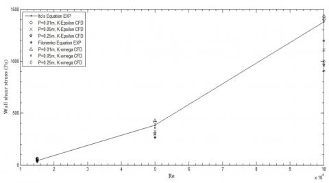
Viewing Figure 11, It can be seen that the difference between the wall shear stress values at Re=15,000 are relatively small and this difference increases as the Reynolds number is increased. The wall shear stress is directly proportional to the Reynolds number; in contrast, the coil friction factor is inversely proportion to the Reynolds number, because the coil friction factor is inversely proportion to the average flow velocity.
Figure 11. Wall shear stress versus Reynolds number using STD $(k-\epsilon)$ model
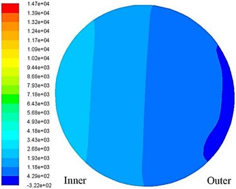
The non-uniformity in pressure distribution becomes more random due to the increment of the turbulence intensity and kinetic energy, particularly near the wall, and thus the inertia of the fluid motion is increased, which enhances the turbulent mixing of the flow regime. The adverse pressure gradient is induced from the curvature of the helically coiled pipe, causing an increment in the pressure near the inner edge of the pipe due to the reduction in fluid particle velocities, while the outer edge will experience an opposite effect [36], as shown in Figure 12 below. For P=0.25m and Re=50,000, the CFD simulation for the third model gives an overestimated result for the wall shear stress, where the pressure difference between the first and second plane was quite high, and consequently leads to a high wall shear stress value, greater than its equivalent at P=0.05m for the same Reynolds number, which is totally wrong, since the STD $(k-\epsilon)$ model presents inadequate performance at severe pressure gradient. Moreover, the wall shear stress for P=0.25m must be lower in comparison with P=0.05m for the same Reynolds number. This error has been corrected by calculating k and epsilon values; and these values have been set in the specification of the inlet boundary conditions instead of intensity and hydraulic diameter. k and epsilon were calculated by using the Eqns. (16) and (17) below [37]:
$k=\frac{2}{3}\left(U \times T_{i}\right)^{2}$ (16)
$\varepsilon=C \mu^{3 / 4} \frac{k^{3 / 2}}{l}$ (17)
Figure 12. Pressure contour of the first plane for P=0.01m at Re=15,000 using STD $(k-\epsilon)$ model
The turbulent kinetic energy and the dissipation rate values have been computed by using the average velocity value for Re=50,000 and $T_{i}$=5% in Eq. (10), which results in k=0.168 (m/sec)2 and $\varepsilon$=32.4 (m2/sec3). This correction gives a reasonably acceptable result for the wall shear stress, as expected, as shown in Figure 13.
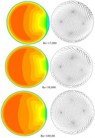
It can be seen that the maximum velocity area increases as the Reynolds number is increased. The velocity profile plays an important role in the unsteadiness of the flow. The turbulent kinetic energy also increases, since it is directly proportion to the flow fluctuating velocity squared. Dean vortices are distorted as the Reynolds number increases due to the high flow velocity which has an effect on Dean vortices configuration, while for P=0.05m, the maximum velocity area is decreased as indicated in Figure 14 but the overall trend seems the same as the first model (P=0.01m) other than velocity magnitude. The streamlines show that the secondary flow intensity increases as the Reynolds number is increased where the distortions in flow paths are clearly indicated in Figure 15.
Figure 13. Velocity contour and vectors of the first plane for P=0.01m using STD $(k-\epsilon)$ model
Figure 14. Velocity contour of the first plane for P=0.05m using STD $(k-\epsilon)$ model
Turning to discuss the velocity contours of the third model (P=0.25m), as a consequence of increasing the pitch size, the influence of the centrifugal forces is highly reduced, which in turn, causes different velocity profile formulations in comparison with the first and second models, as shown in Figure 16.
Figure 17 validates the effect of the centrifugal forces due to the formation of the secondary flow, as explained earlier in the velocity contours section. For P=0.01m, there is a high effect from the secondary flow, which makes the pressure at the inner edge of the pipe relatively high in comparison with its equivalent for P=0.05m and P=0.25m, while for P=0.05m, there is a slightly lower effect of pressure at the inner edge due to the reduction in fluid velocity particles, as indicated in Figure 14. For P=0.25m, the pressure distribution looks quite uniform and this validates that the effect of the secondary flow is almost depleted, which makes the pressure distribution of the third model P=0.25 uniform, as indicated in Figure 17.
In Figure 18, it can be seen that at Re=15,000, the STD $(k-w)$ model predicts higher values of coil friction factor in comparison with the STD $(k-\epsilon)$ model. The STD $(k-w)$ model results are more rigorous in comparison with STD $(k-\epsilon)$ model results. Since the fine mesh is being used in the CFD simulation, a spontaneous transformation is based on $y^{+}$ value from a wall function to a low-Reynolds number approach, consequently giving a more accurate near wall treatment particularly in wall-bounded turbulent flows (Fluent, 2006). Moreover, the STD $(k-w)$ model performs better than the STD $(k-\epsilon)$ model with an adverse pressure gradient and it does not employ a damping function within its configuration.
At Re=50,000 and Re=100,000, both of the models give a satisfactory result where the difference between the results is not more than 0.07% which is acceptable in engineering designs. There are three parameters that have an effect on flow in helically coiled pipe: Dean number, Pitch size, and curvature ratio.
In Figure 19, a comparison of the wall shear stress has been made between the results obtained from the STD $(k-\epsilon)$ and $(k-w)$ models. The STD $(k-\epsilon)$ model predicts high shear stress values in comparison with the STD $(k-w)$ model. In fact, it is hard to recognise the difference in Figure 19 and for this reason, the plot was magnified only for Re=15,000 to show the difference in wall shear stress clearly, as shown in Figure 20.
Figure 15. Vortices formulation for P=0.05m STD $(k-\epsilon)$ model
Figure 16. Velocity contour of the first plane for P=0.25m using STD $(k-\epsilon)$ model
Figure 17. Pressure distribution at Re=15,000 STD $(k-\epsilon)$ model
Figure 18. Friction factor comparison using STD $(k-\epsilon)$ and STD $(k-w)$ model
Figure 19. Wall shear stress comparison using STD $(k-\epsilon)$ and STD $(k-w)$ model
Figure 20. Wall shear stress for Re=15,000 using STD $(k-\epsilon)$ and STD $(k-w)$ model
A comparison has been made between the velocity contours obtained from STD $(k-\epsilon)$ and $(k-w)$ models. Figure 21 shows that the STD $(k-\epsilon)$ model predicts a higher range of velocity, denoted in red, in comparison with the STD $(k-w)$ model. In the STD $(k-\epsilon)$ model, the high-velocity fluid particles fill approximately half of the pipe, which means the effect of the centrifugal forces will also be great and consequently the average pressure value of this plane will be higher than its equivalent in the STD $(k-w)$ model, which explains what was mentioned earlier: that the STD $(k-\epsilon)$ model predicts high shear stress values in comparison with the STD $(k-w)$ model. Increasing the pitch causes a drop in high-velocity fluid particles, which means the effect of the centrifugal forces will be lower, which also causes a drop in pressure gradient within the whole domain, as occurs for P=0.05m in Figure 22 below.
Figure 21. Comparison of the first plane velocity contours for P=0.01m
Figure 22. Comparison of the first plane velocity contours for P=0.05m
In Figure 22, it can be seen that the STD $(k-w)$ model predicts high-velocity values of fluid particles more than its counterpart STD $(k-\epsilon)$ model. The difference in captured velocities magnitude does not exceed 4.7% which is considered acceptable in the CFD field. This difference returns to the configurations and specifications of each turbulence model in terms of accuracy and stability.
Turning to discuss the velocity contours of P=0.25m, it has been found that the maximum velocity values of the whole domain are typical for both turbulence models other than P=0.1m and P=0.05m. However, the velocity distribution in the first plane is not typical, as shown in Figure 23. A small difference in velocity distribution within the planes may cause a high-pressure variation, where the STD $(k-\epsilon)$ model predicts greater high-pressure values than the STD $(k-w)$, which makes the pressure difference between the first and second plane lower in comparison with the STD $(k-w)$ model. As a result, the STD $(k-w)$ model predicts higher wall shear stress values than the STD $(k-\epsilon)$ model, (see Figure 19).
Figure 23. Comparison of the first plane velocity contours for P=0.25m
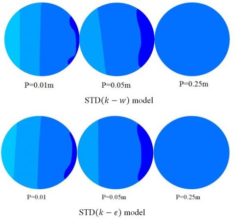
The pressure distribution of the STD $(k-w)$ model does not look very different from that obtained from the STD $(k-\epsilon)$ model, as shown in Figure 24. The remarkable uniform pressure distribution of the STD$(k-w)$ model indicated at P=0.25m gives approximately the same distribution with the STD $(k-\epsilon)$ model, which means that the pitch of the third model is very large to induce high centrifugal forces and formulate an intensive secondary flow.
The pitch size plays a significant role in determination of the secondary flow intensity. Increasing the pitch size has an effect on damping out the turbulent fluctuations in flowing fluid particles, and consequently the emergence of the turbulent flows is delayed in comparison with a straight pipe. For example, the laminar flow in the first model is extended to Reynolds number up to 9581 depending on Ito’s equation.
Figure 24. Comparison of the first plane velocity contours at Re=15,000
In this research, the influence of changing the pitch size was investigated by testing three different models in turbulent flow. This investigation was done through the observation of the coil friction factor profile, wall shear stress, and velocity-pressure contours. Two turbulence models have been utilized: STD(k-ϵ) and STD(k-w) models. It has been found that the STD(k-w) model presents more accurate results in comparison with the STD (k-ϵ) model due to the differences in specifications of the turbulence models in terms of the near wall treatment. However, the STD(k-ϵ) model presents a good estimation for preliminary results. In turbulent flows, Filonenko’s equation was used instead of Colebrook's equation due to the complexity of the Fanning friction factor correlation with the Reynolds number, and it is controlled by Colebrook’s equation. A comparison has been made between the turbulence models to observe the differences in results in terms of coil friction factor and wall shear stress. The found of this study indicated that Dean Number has a stronger effect on reducing coil friction factor than the increment in pitch dimension.
[1] Cioncolini, A., Santini, L. (2006). An experimental investigation regarding the laminar to turbulent flow transition in helically coiled pipes. Experimental Thermal and Fluid Science, 30(4): 367-380. https://doi.org/10.1016/j.expthermflusci.2005.08.005
[2] Ito, H. (1987). Flow in curved pipes. JSME International Journal, 30(262): 543-552. https://doi.org/10.1299/jsme1987.30.543
[3] De Amicis, J., Cammi, A., Colombo, L.P., Colombo, M., Ricotti, M.E. (2014). Experimental and numerical study of the laminar flow in helically coiled pipes. Progress in Nuclear Energy, 76: 206-215. https://doi.org/10.1016/j.pnucene.2014.05.019
[4] Dean, W.R., Hurst, J.M. (1959). Note on the motion of fluid in a curved pipe. Mathematika, 6(1): 77-85. https://doi.org/10.1112/S0025579300001947
[5] Ligrani, P.M. (1994). A study of Dean vortex development and structure in a curved rectangular channel with aspect ratio of 40 at Dean numbers up to 430. Contractor Report.
[6] Austen, D.S., Soliman, H.M. (1988). Laminar flow and heat transfer in helically coiled tubes with substantial pitch. Experimental Thermal and Fluid Science, 1(2): 183-194. https://doi.org/10.1016/0894-1777(88)90035-0
[7] Hüttl, T.J., Friedrich, R. (2000). Influence of curvature and torsion on turbulent flow in helically coiled pipes. International Journal of Heat and Fluid Flow, 21(3): 345-353. https://doi.org/10.1016/S0142-727X(00)00019-9
[8] Yamamoto, K., Yanase, S., Yoshida, T. (1994). Torsion effect on the flow in a helical pipe. Fluid Dynamics Research, 14(5): 259-273.
[9] Hüttl, T.J., Friedrich, R. (2001). Direct numerical simulation of turbulent flows in curved and helically coiled pipes. Computers & Fluids, 30(5): 591-605. https://doi.org/10.1016/S0045-7930(01)00008-1
[10] Castiglia, F., Chiovaro, P., Ciofalo, M., Liberto, M., Maio, P., Piazza, I.D., Giardina, M., Mascari, F., Morana, G., Vella, G. (2010). Modelling flow and heat transfer in helically coiled pipes. Part 3: Assessment of turbulence models, parametrical study and proposed correlations for fully turbulent flow in the case of zero pitch. Report Ricerca di Sistema Elettrico.
[11] Lin, C.X., Ebadian, M.A. (1997). Developing turbulent convective heat transfer in helical pipes. International Journal of Heat and Mass Transfer, 40(16): 3861-3873. https://doi.org/10.1016/S0017-9310(97)00042-2
[12] Rogers, G.F.C., Mayhew, Y.R. (1964). Heat transfer and pressure loss in helically coiled tubes with turbulent flow. International Journal of Heat and Mass Transfer, 7(11): 1207-1216. https://doi.org/10.1016/0017-9310(64)90062-6
[13] Yang, G., Ebadian, M.A. (1996). Turbulent forced convection in a helicoidal pipe with substantial pitch. International Journal of Heat and Mass Transfer, 39(10): 2015-2022. https://doi.org/10.1016/0017-9310(95)00303-7
[14] Mori, Y., Nakayama, W. (1967). Study on forced convective heat transfer in curved pipes: (3rd report, theoretical analysis under the condition of uniform wall temperature and practical formulae). International Journal of Heat and Mass Transfer, 10(5): 681-695. https://doi.org/10.1016/0017-9310(67)90113-5
[15] Kirpikov, A.V. (1957). Heat transfer in helically coiled pipes. Trudi. Moscov. Inst. Khim. Mashinojtrojenija, 12: 43-56.
[16] Seban, R.A., McLaughlin, E.F. (1963). Heat transfer in tube coils with laminar and turbulent flow. International Journal of Heat and Mass Transfer, 6(5): 387-395. https://doi.org/10.1016/0017-9310(63)90100-5
[17] Bai, B., Guo, L., Feng, Z., Chen, X. (1999). Turbulent heat transfer in a horizontal helically coiled tube. Heat Transfer-Asian Research: Co-sponsored by the Society of Chemical Engineers of Japan and the Heat Transfer Division of ASME, 28(5): 395-403. https://doi.org/10.1002/(SICI)1523-1496(1999)28:5<395::AID-HTJ5>3.0.CO;2-Y
[18] Ali, S. (2001). Pressure drop correlations for flow through regular helical coil tubes. Fluid Dynamics Research, 28(4): 295-310.
[19] Kedzierski, M., Kim, M.S. (1996). Single-phase heat transfer and pressure drop characteristics of an integral-spine fin within an annulus. Journal of Enhanced Heat Transfer, 3(3): 201-210. https://doi.org/10.1615/JEnhHeatTransf.v3.i3.40
[20] White, C.M. (1929). Streamline flow through curved pipes. Proceedings of the Royal Society of London. Series A, Containing Papers of a Mathematical and Physical Character, 123(792): 645-663. https://doi.org/10.1098/rspa.1929.0089
[21] White, C.M. (1932). Fluid friction and its relation to heat transfer. Trans. Inst. Chem. Eng. (London), 10: 66-86.
[22] Prandtl, L. (1949). Fuhrer dmchdie Stromungslehre, 3rd Edition, 159, Braunsschweigh; English Transl., Essentials of Fluid Dynamics, Blackie and Son, London, 168.
[23] Adler, M. (1934). Strömung in gekrümmten Rohren. ZAMM-Journal of Applied Mathematics and Mechanics/Zeitschrift für Angewandte Mathematik und Mechanik, 14(5): 257-275.
[24] Hasson, D. (1955). Streamline flow resistance in coils. Res. Corresp, 1: S1.
[25] Mishra, P., Gupta, S.N. (1979). Momentum transfer in curved pipes. 1. Newtonian fluids. Industrial & Engineering Chemistry Process Design and Development, 18(1): 130-137. https://doi.org/10.1021/i260069a017
[26] Patankar, S.V., Spalding, D.B. (1972). A calculation procedure for heat, mass and momentum transfer in three-dimensional parabolic flows. International Journal of Heat and Mass Transfer, 15(10): 1787-1806. https://doi.org/10.1016/0017-9310(72)90054-3
[27] Chou, P.Y. (1945). On velocity correlations and the solutions of the equations of turbulent fluctuation. Quarterly of Applied Mathematics, 3(1): 38-54.
[28] Harlow, F.H., Nakayama, P.I. (1968). Transport of turbulence energy decay rate (No. LA-3854). Los Alamos Scientific Lab., N. Mex.
[29] Davidov, B.I. (1961). On the statistical dynamics of an incompressive fluid. Doklady Academy Nauka SSSR, 136: 47.
[30] Jones, W.P., Launder, B.E. (1972). The prediction of laminarization with a two-equation model of turbulence. International Journal of Heat and Mass Transfer, 15(2): 301-314.
[31] Launder, B.E., Sharma, B.I. (1974). Application of the energy-dissipation model of turbulence to the calculation of flow near a spinning disc. Letters in Heat and Mass Transfer, 1(2): 131-137.
[32] Wilcox, D.C. (1988). Turbulence Modeling for CFD. DCW Industries., United States.
[33] Launder, B.E., Morse, A., Rodi, W., Spalding, D.B. (1973). Prediction of free shear flows: A comparison of the performance of six turbulence models. NASA. Langley Res. Center Free Turbulent Shear Flows.
[34] Colebrook, C.F., White, C.M. (1937). Experiments with fluid friction in roughened pipes. Proceedings of the Royal Society of London. Series A-Mathematical and Physical Sciences, 161(906): 367-381. https://doi.org/10.1098/rspa.1937.0150
[35] Menter, F. (1993). Zonal two equation kw turbulence models for aerodynamic flows. 23rd Fluid Dynamics, Plasmadynamics, and Lasers Conference. https://doi.org/10.2514/6.1993-2906
[36] Kalpakli, A. (2012). Experimental study of turbulent flows through pipe bends. Doctoral dissertation, KTH Royal Institute of Technology.
[37] Versteeg, H.K., Malalasekera, W. (2007). An introduction to computational fluid dynamics: The finite volume method. Pearson education.