Nabeel Abu Shaban | Ibraheem Nasser | Jamil Al Asfar* | Safwan Al-Qawabah | Abdullah N. Olimat
© 2020 IIETA. This article is published by IIETA and is licensed under the CC BY 4.0 license (http://creativecommons.org/licenses/by/4.0/).
OPEN ACCESS
In this study, energy and exergy analysis was performed for a refrigerator display cabinet (RDC) unit equipped with a variable speed DC-compressor and electronic expansion valve. Economic impact and energy saving were also investigated. Two identical refrigeration systems were built and tested experimentally to find the most efficient and feasible one. The first system was built using the existing commercial way of building up the refrigeration cycle of the RDC unit using an on/off switch for the compressor, and mechanical traditional thermal expansion valve (TEV). The other system was equipped with a variable refrigerant flow (VRF) DC-compressor, with inverter and electronic expansion valve (EEV) instead of the mechanical expansion valve. Complete specifications of each component and measurement devices used in this work are included in this study. It was found that the new RDC unit equipped with the VRF system provided 32% energy saving, and less exergy destruction than the commercial cabinet. So, the use of the new suggested RDC units will reduce the energy bill of such sector by 32%.
thermodynamics, VRF, DC compressor, electronic expansion valve, refrigerator
The use of an RDC unit for food preservation and display is an intensive energy-consuming process. The saving in energy consumption is an important issue in the development and design of all cooling processes. The compressor which is at the heart of the cooling process represents the most energy consuming part. Thus, a better-quality compressor will reduce energy consumption which is always required. RDCs play a vital role in food preservation around the world, where compliance with food display requirements is a prerequisite for taking advantage of market share competition and opportunities. Shopping malls, shops and retail markets increasingly need to use RDCs to offer a wide range of food product displays.
In recent years, much research has concentrated on energy savings in thermal systems to produce more energy saving systems without affecting performance. Refrigeration and air conditioning systems consume a lot of power in industrial applications. Furthermore, most air conditioning companies tend to use VRF technology in their systems to minimise power consumption and increase efficiency.
VRF refers to the ability of a system to control the rate of refrigerant flow to each evaporator. This will enable the supply of many evaporators of different capacities and configurations, individualised comfort control, simultaneous heating and cooling in different zones, and heat recovery from one zone to another.
A VRF air conditioning system is a technology improved by commercial companies. The updated technology in VRF systems offers a great scale of energy efficiency; these systems operate quietly and provide the user with full control of environmental temperatures. Traditional HVAC systems are often limited to one condensing unit, one compressor and one evaporator, while a VRF system is designed to specifically meet the needs of several independent consumers inside one commercial mall or building. One condensing unit can be connected to several evaporators, each of which is individually controlled.
Exergy analysis for a theoretical vapour compression refrigeration cycle utilizing R12, R22 and R134A was analysed by Khan et al. [1]. The investigations showed that various results were obtained for the effect of evaporating temperatures on COP and exergetic efficiency. Performance parameters such as entropy generation, COP and exergetic efficiency were investigated at different ambient conditions by Chopra et al. [2] for different refrigerants such as R152a, R600, R600a, R410a, R290, R1234yf, R404a and R134a. It was found that both the energy and exergy efficiencies of R134a are 8.97% and 5.38% lower than R152a and R600 respectively at -50℃ evaporating and 45℃ condensing temperatures. The exergetic analysis of an R134A-based actual vapour compression refrigeration cycle was presented by Yadav et al. [3]. The component’s exergetic destruction and the cycle’s exergetic efficiency were found. A detailed exergy analysis for a theoretical vapour compression refrigeration cycle using R404A, R407C and R410A was studied by Soni1 and Gupt [4]. A detailed experimental analysis of a 2TR (ton of refrigeration) vapour compression refrigeration cycle for different percentages of refrigerant charge using exergy analysis was presented by Anand and Tyagi [5]. Application of the two-phase ejector in a subcritical refrigeration system was discussed by Dudar et al. [6]. Results of exergy analysis of the system operating with various working fluids for various operating conditions were studied. Their study showed a possible exergy efficiency increase in the refrigeration compression cycle. Exergy analysis of a transcritical carbon dioxide refrigeration cycle with an expander was performed by Yang et al. [7] and an exergetic analysis on a vapour compression refrigerating system was described by Xu and Clodic [8]. Effect of pressure drop and longitudinal conduction on exergy destruction in a concentric-tube micro-fin tube heat exchanger is studied by Imteyaz and Zubair [9]. Different types of refrigerants such as R404A, R134A, R22, and R410A were investigated for different single as well as multi-stage systems of vapour compression refrigeration cycles by Morad et al. [10]. The differences in the thermal and mechanical exergies in each component of air-cooled air conditioning system were analyzed by Yoo et al. [11].
Based on above, and according to author’s best knowledge, no detailed thermodynamic analysis of an RDC unit was done using experimental data. In this study, the performance of a variable speed rotary compression controlled by a DC frequency inverter will be presented.
Compressor performance has been analysed by many researchers, but most assume that the compressor runs at a constant conventional speed. The main issue in this work is to study the effects of compressor performance under different speeds. Thus, the performance of the compressor may be improved, leading to achieve best energy saving and less exergy destruction.
Another issue will be discussed in this study, which is the electronic expansion valve performance. EEV controls the flow of refrigerant entering a direct expansion evaporator. It does this in response to signals sent by an electronic controller. Most companies try to change the old system to a new system using an electronic expansion valve instead of a mechanical one. Improving the performance of the EEV will in turn improve the efficiency of the refrigeration system as a result.
In this work, performance enhancement, thermodynamic analysis and energy saving for fridge cabinets will be investigated. A refrigeration cycle will be presented and analyzed to enhance its performance. A new proposed system that can really minimize power consumption will be built. The new proposed system will be equipped with a DC compressor instead of a constant speed compressor, and an EEV electronic expansion valve instead of a mechanical expansion valve.
3.1 External cooling load
One chiller cabinet will be used in this study. The dimensions of the open-front refrigerated display cabinet are 1.83m long, 0.586m wide and 1.435m high. The ambient air is 25℃ at 50% RH, the internal air is 2℃ at 50% RH. The roof and floor walls are all insulated with 45mm polyurethane which has a thermal conductivity value 0.023 W/m.K. The overall heat transfer coefficient is calculated using Fourier's law. The following equations are used to calculate the overall heat transfer coefficient of walls. [12]:
$U=\frac{1}{R_{t h}}$ (1)
$R_{t h}=R_{0}+\sum_{1}^{n} \frac{x_{n}}{k_{n}}+R_{i}$ (2)
$R_{t h}=0.10+\frac{0.045}{0.023}+0.12=2.17 \mathrm{m}^{2} . \mathrm{K} / \mathrm{W}$
$U=\frac{1}{R_{t h}}=\frac{1}{2.17}=0.46 \mathrm{W} / \mathrm{m}^{2} \cdot \mathrm{K}$
The ground temperature of the refrigerator is assumed 2℃. Typical value of the convection heat transfer coefficient (h) is (2-25) W/m2.K and its value will be assumed 10 W/m2.K. To calculate the transmission load, the conduction and convection heat transfer formula is used by Incropera [12]:
For conduction
$Q=U \times A\left(T_{0}-T_{i}\right)$ (3)
For convection
$Q=h \times A\left(T_{a}-T_{i}\right)$ (4)
The dimension of the RDC unit used in this work is shown in the following Table 1.
Table 1. RDC dimension
|
Face |
Length (m) |
Width (m) |
Area (m2) |
|
Left Side |
1.435 |
0.586 |
0.841 |
|
Right Side |
1.435 |
0.586 |
0.841 |
|
Roof |
1.830 |
0.586 |
1.072 |
|
Bottom |
1.830 |
0.586 |
1.072 |
|
Back side |
1.830 |
1.435 |
2.262 |
|
Front side |
1.830 |
1.435 |
2.262 |
On the front side, the convection formula is used because heat losses here will be between the inside cold air and outside hot air, and Table 3 shows the convection heat loss from the front freezer side.
Table 2. The evaporator conduction load from walls
|
|
A (m2) |
U (W/m2.K) |
ΔT (${ }^{\circ} \mathrm{C}$) |
Q (W) |
|
Left Side |
0.841 |
0.46 |
(25-2) |
8.9 |
|
Right Side |
0.841 |
0.46 |
(25-2) |
8.9 |
|
Roof |
1.072 |
0.46 |
(25-2) |
11.3 |
|
Bottom |
1.072 |
0.46 |
(25-2) |
11.3 |
|
Back side |
2.262 |
0.46 |
(25-2) |
23.9 |
|
|
A (m2) |
h (W/m2.) |
ΔT (${ }^{\circ} \mathrm{C}$) |
Q (W) |
|
Front Side |
2.262 |
10 |
(25-2) |
520.3 |
The cooling load from the product exchange is calculated as being the heat brought into the refrigerator from new products which are at a higher temperature.
The freezer is used to store cheese; approximately 250 kg of cheese arrive each day divided by 14 hours at a temperature of 10℃ and a specific heat capacity of cheese is 2.15 kJ/ kg.℃.
The heat exchange formula is used for heating capacity losses from cheese to freezer
$\begin{aligned} Q &=(250 \mathrm{kg} / 14 \mathrm{h}) \times 2.15 \mathrm{kJ} / \mathrm{kg} \cdot{ }^{\circ} \mathrm{C} \times\left(10^{\circ} \mathrm{C}-2^{\circ} \mathrm{C}\right) \\ &=5.11 \mathrm{kW} \end{aligned}$
3.2 Internal heat load
The heat generated by the lighting is calculated using the lighting heating load formula:
Q= n x t, W (5)
If two LED lamps of 18W-power each are used, the heat will be:
Q= 2 x 18W = 36 W
In this refrigerator, the evaporator, with two fans rated at 10W each, the heat generated by the fan motors in the evaporator will be:
Q = 2 x 10W = 20 W
3.3 Total cooling load
To calculate the total cooling load, we add all the calculated values to get:
Transmission load: 0.064 kW
Convection load: 0.520 Kw
Product load: 5.110 kW
Internal load: 0.036 kW
Equipment load: 0.020 kW
Total = 5.75 kW
A safety factor of (5%) should be applied to account for errors and possible variations from design point. Thus,
The total load will be 5.75 x1.05 = 6.0 kW = 1.7 TR.
3.4 Refrigeration cycle
Figure 1. Schematic drawing of vapor compression refrigeration cycle
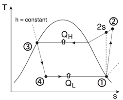
The vapor-compression refrigeration cycle is the common cycle used for refrigerators and air conditioning systems. Figure 1 shows the main components of a refrigeration cycle, which are compressor, condenser, evaporator and expansion valve, which are classified into two types: traditional and electronic expansion valves are shown in Figure 3. Figure 2 shows the main processes of the ideal vapour-compression refrigeration cycle on T-s diagram, and it consists of four processes:
1-2 Isentropic compression in a compressor.
2-3 Constant-pressure heat rejection in a condenser.
3-4 Throttling in an expansion device.
4-1 Constant-pressure heat absorption in an evaporator.
Figure 2. T-s diagram for the ideal vapor-compression refrigeration cycle
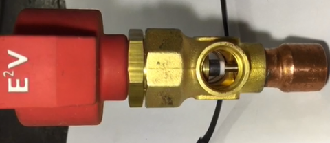
Figure 3. Electronic expansion valve
3.5 Mollier (h-s) chart of the ref. R404a
The following values and parameters, specified below, are selected from the Mollier chart of the refrigerant R404a for the operating pressure range of 4.3913 bars to 18.2 bars for the design of a display cabinet refrigerator structure for 250kg of cheese.
h1= 362.6 kJ/kg s1= 1.6202 kJ/kg.K
h2s = 386.15 kJ/kg s2= 1.6202 kJ/kg.K
h3= 242.6 kJ/kg s3= 1.1465 kJ/kg.K
h4= 242.6 kJ/kg s4= 1.1636 kJ/kg.K
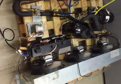
The details and specification of the vapor-compression refrigeration components shown in Figure 4 and measurement devices of all tested systems, including compressor, VRF, evaporator, invertor and condenser are summarized in Table 4. All the measurement devices used in this study have been calibrated before installing them.
Table 4. Device, tools, and components of refrigeration cycle
|
Item |
Usage |
|
Reciprocating compressor |
To increase the pressure of the refrigerant and reduce its volume |
|
Dc compressor |
To increase the pressure of the refrigerant and reduce its volume |
|
Electronic expansion valve EEV |
A metering device designed to regulate the rate at which liquid refrigerant flows into evaporator |
|
Mechanical expansion valve TEV |
A metering device designed to regulate the rate at which liquid refrigerant flows into evaporator |
|
Evaporator |
It used to extract heat from the chamber where temperature maintenance is required |
|
Condenser |
Used for taking latent heat of fluid and converting it into liquid form |
|
Filter dryer |
Used to trap the moisture, small metal chips and dirt in the refrigerant |
|
Low-pressure transmitter sensor |
To measure the low pressure |
|
High-pressure transmitter sensor |
To measure the high pressure |
|
Data logger |
To collect history data of temperature and pressure sensor |
|
Temperature sensor |
To measure the evaporator and condenser temperature |
|
Temperature controller |
Used to read and control the set point temperature |
|
Rack system controller |
To read the high and low pressure |
|
Power meter |
To accumulate the power consumed per day |
|
Refrigerant. R404a |
Used as refrigerant gas |
|
Display cabinet refrigerator |
Refrigerator |
Figure 4. The vapor-compression refrigeration cycle
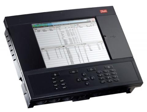
Figure 5. A Danfoss data logger device
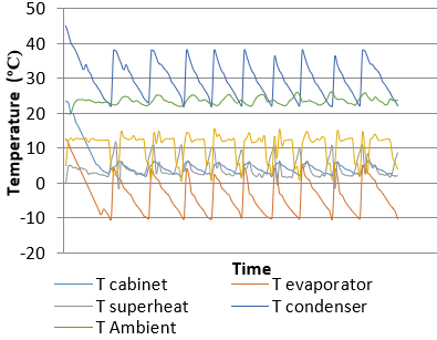
Figure 6. The temperature response of all collected temperatures in traditional system
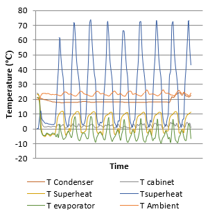
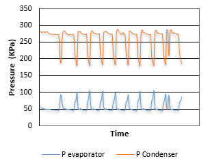
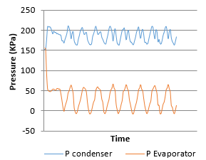
A Danfoss data logger which is shown in Figure 5; was used to accumulate the required parameters. Condenser, evaporator temperatures and pressures are recorded and uploaded as an Excel sheet to take the actual results and use in the project. The Figures 6-10 represent the actual reading of (Te, Tc, Pe, Pc, T super heat) for the economy VRF and traditional systems, which are collected from the installed data logger the rate of the sample was 2 minutes.
Figure 7. The temperature response of all collected temperatures when VRF is installed
Figure 8. The evaporator and condenser pressure for 24 hours in traditional system
Figure 9. The evaporator and condenser pressure for 24 hours when VRF is installed
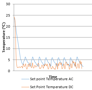
Figure 10. Set point temperature for AC and DC compressors
The vapor-compression refrigeration cycle is operating between a low-temperature reservoir at TL and a high-temperature reservoir at TH. The maximum COP of a refrigeration cycle operating between temperature limits is given by Çengel [13].
$\operatorname{COP}_{R-C}=\frac{T_{L}}{T_{H}-T_{L}}$ (6)
Exergy destruction for major components of a refrigeration system is written as follows:-
Compressor:
$\dot{X}_{\text {dest}, 1-2}=T_{\mathrm{o}} \dot{S}_{g e n, 1-2}=\dot{m} T_{\mathrm{o}}\left(s_{2}-s_{1}\right)$ (7)
Condenser:
$\dot{X}_{\text {dest}, 2-3}=T_{\mathrm{o}} \dot{S}_{g e n, 2-3}=T_{\mathrm{o}}\left[\dot{m}\left(s_{3}-s_{2}\right)+\frac{\dot{Q}_{H}}{T_{H}}\right]$ (8)
Expansion Valve:
$\dot{X}_{\text {dest}, 3-4}=T_{\mathrm{o}} \dot{S}_{\text {qen}, 3-4}=\dot{m} T_{\mathrm{o}}\left(s_{4}-s_{3}\right)$ (9)
Evaporator:
$\dot{X}_{\text {dest}, 4-1}=T_{\mathrm{o}} \dot{S}_{g e n, 4-1}=T_{0}\left[\dot{m}\left(s_{1}-s_{4}\right)+\frac{\dot{Q}_{L}}{T_{L}}\right]$ (10)
The total energy destruction associated with the refrigeration cycle is the summation of the energy destruction for each component of the cycle:
$\dot{X}_{\text {dest}, \text {total}}=\dot{X}_{\text {dest}, 1-2}+\dot{X}_{\text {dest}, 2-3}+\dot{X}_{\text {dest}, 3-4}+\dot{X}_{\text {dest}, 4-1}$ (11)
The second law of efficiency (Exergy Efficiency) of the refrigeration cycle is equal to the ratio of actual COP to maximum COP for the cycle:
$\eta_{I I}=\frac{C O P_{R}}{C O P_{R-C}}$ (12)
The actual power consumption for a continuous 20-hour operation of the refrigerator for both systems. For the traditional cycle, the start-reading was 1292.5 kW/h, while the final reading was 1018 kW/h, and the total power consumed was 25.3 kW/20h. Whereas VRF system start- reading was 1254 kW/h, while the final reading was 1271.1 kW/h, and the total power consumed was 17 kW/20h.
To find the percentage of energy saving between the systems use this equation:
$\begin{aligned} \text {saving } \%=& \frac{\text {traditional}(k W)-V R F(k W)}{\text {traditional}(k W)} \times 100 \% \end{aligned}=\frac{25.3-17}{25.3} \times 100 \%=32.8 \%$
This means that 32% energy saving was achieved when using a DC compressor and EEV.
Regarding the operating pressure and temperature, it is noticed that the evaporator and condenser for the VRF system were 25 kPa and 175 kPa, compared with 75 kPa and 230 kPa for the traditional system. This reduction minimizes the VRF compressor input work, resulting in higher second law efficiency. The temperature of the condenser and evaporator show that both systems kept cold space at -5°C.
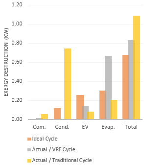
Figure 11. Exergy destruction for different components of the refrigeration cycle for ideal, VRF and Traditional cycles
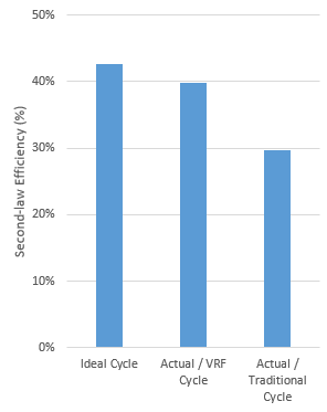
Figure 11 shows the exergy destruction for the compressor, condenser, evaporator, expansion valves and for the refrigeration cycle for the ideal cycle, VRF system and traditional system. Figure 12 shows the percentage of exergy destruction for every component (as ratio to total exergy destruction in complete cycle) for different cycles, and the second law efficiency is presented in Figure 13.
Figure 12. Exergy destruction percentage for different components of the refrigeration cycle for ideal, VRF and Traditional cycles
Figure 13. Exergy efficiency of the refrigeration cycle for ideal, VRF and Traditional cycles
The error or uncertainty analysis in an experimental work quantifies the difference between measured and true value of a thermo physical quantity of a material. The uncertainty in the estimate of the true value provides a rational way of evaluating the significance of the scatter on repeated trials [14].
$C O P_{R-C}=f\left(T_{L}, T_{H}\right)$ (13)
$\Delta C O P_{R-C}=\sqrt{\left(\frac{\partial C O P_{R-C}}{\partial T_{L}} \cdot \Delta T_{L}\right)^{2}+\left(\frac{\partial C O P_{R-C}}{\partial T_{H}} \cdot \Delta T_{H}\right)^{2}}$ (14)
where,
$\frac{\partial C O P_{R-C}}{\partial T_{L}}=\frac{T_{H}}{\left(T_{H}-T_{L}\right)^{2}}$ (15)
$\frac{\partial C O P_{R-C}}{\partial T_{H}}=\frac{-T_{L}}{\left(T_{H}-T_{L}\right)^{2}}$ (16)
From Table 5, the actual evaporative and condenser temperature are -6.2℃ and 29.9℃, respectively. $\Delta T_{L}=\Delta T_{H}=0.1^{\circ} \mathrm{C}$. Substituting in Eqns. (14), (15) and (16):
$\begin{aligned} \operatorname{COP}_{R-c}=7.4 \text { and } & \Delta C O P_{R-\text {Carnot}} =& 0.030973 \end{aligned}$
The percentage of uncertainty in evaluating $C O P_{R-C}$ of traditional cycle is:
$\begin{aligned} \frac{\Delta C O P_{R}-C}{C O P_{R-C}} \times 100 \% &=\frac{0.030973}{7.4} \times 100 \% =\pm 0.42 \% \end{aligned}$
From Table 5, the actual evaporative and condenser temperature are -7℃ and 18.9℃, respectively. $\Delta T_{L}=\Delta T_{H}=0.1^{\circ} \mathrm{C}$. Substituting in Eqns. (14), (15) and (16).
$\begin{aligned} \operatorname{COP}_{R-c}=10.3 & \text { and } \Delta C O P_{R} \text { -Carnot } =0.058872 \end{aligned}$
The percentage of uncertainty in evaluating $C O P_{R-C}$ of VRF system is:
$\begin{aligned} \frac{\Delta C O P_{R}-C}{C O P_{R-C}} \times 100 \% &=\frac{0.058872}{10.3} \times 100 \% =\pm 0.57 \% \end{aligned}$
Table 5. The required parameters which are collected from Danfoss data logger
|
Parameter name |
Unit |
Traditional cycle |
VRF system |
|
Time to reach from 23°C to 2°C |
min |
36 |
12 |
|
Power consumption\20 h |
kWh |
25.3 |
17 |
|
Actual Evaporator Temperature [TL] (Avg) |
˚C |
-6.2 |
-7 |
|
Actual Condenser Temperature [TH] (Avg) |
˚C |
29.9 |
18.9 |
|
Compressor power |
W |
1460 |
1300 |
|
Ambient temperature for air [TO] |
˚C |
23.3 |
23.7 |
|
Low pressure (Avg) |
bar |
5.68 |
3.26 |
|
High pressure (Avg) |
bar |
25.84 |
18.61 |
|
Mass flow rate |
kg/s |
0.05 |
0.05 |
|
Set point temperature avg. |
˚C |
2.2 |
5.1 |
In this work, it has been shown that RDC unit equipped with a VRF DC compressor has minimum exergy destruction when compared with the traditional system. Furthermore, exergy destruction in the condenser was almost eliminated, whereas exergy destruction in the evaporator has been increased. The RDC with VRF system provides 32% energy saving, and 76% less exergy destruction than the conventional system. EEV provides precise state of superheat to minimum possible level, while the evaporator is also charged optimally. Both of these optimal operations lead the compressor to work within optimal conditions; therefore, the work needed for operating the compressor will be minimum, Thus, energy saving reaches the highest rate.
|
k |
The thermal conductivity [W/m.K] |
|
Rth |
Thermal resistance [m2.K/W] |
|
Ro |
Inside film resistance [m2.K/W] |
|
Ri |
Outside film resistance [m2.K/W] |
|
Q |
Heat Transfer [W] |
|
U |
Overall heat transfer coefficient [W/m2.K]. |
|
A |
Area [m2] |
|
TL TH To |
Evaporator Temperature [°C] Condenser Temperature [°C] Ambient temperature for air [°C] |
|
RH |
Relative Humidity |
|
N |
Number of Lambs |
|
t |
Time [s] |
|
h |
Enthalpy[kJ/kg] |
|
S |
Entropy[kJ/kg.s] |
|
$\dot{Q}_{H}$ |
Cold medium heat [W] |
|
$\dot{Q}_{L}$ |
Warm medium heat [W] |
|
$\dot{m}$ |
Mass flow rate of the ref. R404a [kg/s] |
|
$\mathrm{COP}_{\mathrm{R}-\mathrm{C}}$ |
Coefficient of performance of Carnot cycle |
|
$C O P_{R . r e v}$ |
Coefficient of performance of reversible cycle |
|
$\dot{X}_{\text {dest}}$ |
Exergy destruction [W] |
|
$\eta_{I I}$ |
Exergy Efficiency or 2nd law of Efficiency |
[1] Khan, N., Khan, M., Ashar, M., Khan, A.Z. (2015). Energy and exergy analysis of vapour compression refrigeration system with R12, R22, R134a. International Journal of Emerging Technology and Advanced Engineering, 5(3).
[2] Chopra, K., Sahni, V., Mishra, R.S. (2015). Energy, exergy and sustainability analysis of two-stage vapour compression refrigeration system. Journal of Thermal Engineering, 1(4): 440-445. https://doi.org/10.18186/jte.95418
[3] Yadav, P., Sharma, A. (2016). Exergy analysis of R134a based vapour compression refrigeration tutor. Journal of Mechanical and Civil Engineering, 2278-1684
[4] Res, R., Soni, J., GuptaJyoti Soni, R.C., Gupta, R.C. (2013). Performance analysis of vapour compression refrigeration system with R404A, R407C and R410A. International Journal of Mechanical Engineering & Robotics Research, 2(1): 25-36.
[5] Anand, S., Tyagi, S.K. (2012). Exergy analysis and experimental study of a vapor compression refrigeration cycle. Journal of Thermal Analysis and Calorimetry, 110: 961–971. https://doi.org/10.1007/s10973-011-1904-z
[6] Dudar, A., Butrymowicz, D., Smierciew, K., Karwacki, J. (2013). Exergy analysis of operation of two-phase ejector in compression refrigeration systems. Archives of Thermodynamics, 34(4): 107–122.
[7] Yang, J.L., Ma, Y.T., Li, M.X., Guan, H.Q. (2005). Exergy analysis of transcritical carbon dioxide refrigeration cycle with an expander. Energy, 30(7): 1162–1175. https://doi.org/10.1016/j.energy.2004.08.007
[8] Xu, X., Clodic, D. (1992). Exergy analysis on a vapor compression refrigerating system using R12, R134a and R290 as refrigerants. International Refrigeration and Air Conditioning Conference, Purdue University Purdue e-Pubs.
[9] Imteyaz, B., Zubair, S.M. (2018). Effect of pressure drop and longitudinal conduction on exergy destruction in a concentric-tube micro-fin tube heat exchanger. International Journal of Exergy, 25(1): 75-91. https://doi.org/10.1504/IJEX.2018.088888
[10] Morad, B., Gadalla, M., Ahmed, S. (2018). Energetic and exergetic comparative analysis of advanced vapour compression cycles for cooling applications using alternative refrigerants. International Journal of Exergy, 26(1-2): 226–246. https://doi.org/10.1504/IJEX.2018.092524
[11] Yoo, Y., Oh, H.S., Uysal, C., Kwak, H.Y. (2018). Thermoeconomic diagnosis of an air-cooled air conditioning system. International Journal of Exergy, 26(4): 393-417. https://doi.org/10.1504/IJEX.2018.10014405
[12] Incropera, F.P. (2011). Fundamentals of Heat and Mass Transfer (7th ed.). John Wiley, Hoboken, NJ.
[13] Çengel, Y. (2008). Thermodynamics: An Engineering Approach. Boston: McGraw-Hill Higher Education.
[14] Holman, J. (2012). Experimental Methods for Engineers. McGraw-Hill Hill Higher Education, London.