Chukwunonso F. Nwoye* | Chukwuemeka H. Otamiri
© 2020 IIETA. This article is published by IIETA and is licensed under the CC BY 4.0 license (http://creativecommons.org/licenses/by/4.0/).
OPEN ACCESS
Regenerators are essential component of systems such as Stirling engines, gas turbines and even IC engines. Designing compact and high performance regenerative system however is quite difficult and has impeded the development of engines such as Stirling engine despite its multifuel capability and potential of reducing the dominance of fossil fuel as a primary energy source. Here the Flow dynamics through regenerators defined by channel matrix geometry and how they impact on convective heat transfer and pressure losses in the system were studied for 0.01<Re<950 using ANSYS FLUENT. Ten values of Re were considered within this range for three matrix geometries-sphere, cube and diamond. Heat transfer in the systems were strongly influenced by the area of convective heat transfer surface, scale of vortex formed and the thermal boundary layer thickness developed from the point of flow separation. The friction coefficient which measures the pressure losses were found to be proportional to the size of the wake or recirculating region downstream of the flow. The suitability of a geometry for use in regenerator matrix design was determined by the ratio of to heat transfer per unit area of matrix. The sphere and diamond matrix gave a similar and better performance than the cube for the range of Re considered.
CFD, convective heat transfer, regenerator, matrix geometry, pressure losses, Stirling engine, friction coefficient
Harnessing alternative energy resources has generated intense global interest in recent times. This is partly due to vulnerabilities associated with sole dependency on fossil fuel for the worlds growing energy need and the compelling need to control greenhouse gas emissions particularly CO2 of which 75% of its concentration in the atmosphere is estimated to come from fossil fuel [1]. In addition to availability of cost effective technology for converting fossil fuel to useful work, other of its appeals include availability, spread, variety of form, transportability and social acceptance. Breaking the dominance of fossil fuel as a primary energy source therefore requires that the alternatives should at least offer comparative prospect. Stirling engine with its relatively high efficiency and multifuel capability holds such potential [2].
Stirling engine operations involves the expansion of hot working fluid (gas) in the hot cylinder as heat is supplied externally. The expanded hot gas passes through a regenerator (where some of its thermal energy is extracted and stored) to the cold space. In the cold space, the gas is compressed by the displacer piston and routed back to the regenerator where the stored heat energy is released back to it. This heat release and extraction in the regenerator are accomplished ideally and reversibly [3].
By periodic extraction and release of heat from the working fluid by the regenerator as it moves in the cycle through the engine, the heat energy that would have been lost in the process is conserved. Therefore the effectiveness of the regenerator significantly influence the overall efficiency of the engine. A good regenerator must be thermally effective, have low flow resistance and low conduction losses [4]. Difficulty in designing a regenerator of reasonable size that meets this criteria and yet stable at high temperature is a major setback in the success of Stirling engine [5].
The motivation of this study is to improve on the effectiveness of regenerators for use in Stirling engines. The focus was on CFD simulation of flow dynamics occasioned by variation in regenerator matrix geometry and their impact on heat transfer and pressure losses in the system.
To study the performance of a regenerator, Faruoli et al., [6] simulated the thermo-fluid behavior using OpenFOAM code.
Liu [7] developed a transient numerical model from experimental procedure to predict the performance of a passive regenerator while Maria et al. [8] simulated regenerator matrix as a porous block. This, though allowed for an approximation of the overall behavior of the system, came at the expense of detailed knowledge of the systems flow dynamics.
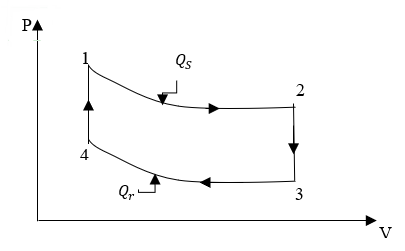
Stirling cycle is a reversible closed cycle that consists of two isothermal and two isochoric processes and can be represented on PV diagram as shown in Figure 1 [5].
In process 1-2 the working fluid expands isothermally in the cylinder as heat is supplied externally. The expanded gas passes through the regenerator in process 2-3 where heat is extracted from the fluid at constant volume and stored. The cold gas in state 3 is compressed to state 4 at constant temperature and in process 4-1, the compressed gas is passed through the regenerator were the stored heat is transferred back at constant volume.
Figure 1. Stirling cycle
Ideally, the heat supply to the system ($Q_{s}$) from the external source is that added isothermally from state 1-2 and heat rejected ($Q_{r}$) is that rejected isothermally from state 3-4 hence the efficiency of a Stirling cycle and heat transfer in the regenerator respectively are given as Eq. (1) . and Eq. (2) [5].
$\eta_{t h}=1-\frac{T_{r}}{T_{s}}$
$T_{r}=T_{3}=T_{4}$
$T_{S}=T_{1}=T_{2}$ (1)
Also
$C_{v}\left(T_{2}-T_{3}\right)=C_{v}\left(T_{1}-T_{4}\right)$ (2)
Eq. (1). is the same as Carnot cycle efficiency which is the highest possible theoretical efficiency of a heat engine operating between two temperatures. The actual efficiency of a Stirling engine is about 20-60% of this [4] with the departure coming from friction losses and thermal irreversibilities in the system [9]. Similarly, achieving high system temperature necessary for improved efficiency is constrained by material limitations, while the desired low regenerator exit temperature requires an increased surface area which introduces friction into the system with resultant undesirable pressure drop [10].
The improved heat transfer in a regenerator can be achieved using porous medium due to high surface area to volume ratio [11]. Maria et al. [8], Kuldeep and Kesarwani [12] and Falk [13] analysed the heat transfer and fluid flow in regenerators by considering the fixed matrix bed as a porous medium.
The performance of a regenerator is measured by pressure drop in the system and its ability to exchange heat with the working fluid [6, 7]. This depends on the thermal properties of the regenerator matrix and flow channel architecture [4]. Heat exchange between a working fluid and regenerator matrix at different temperatures as the fluid flows through the matrix is given by Eq. (3) [14, 15].
$Q_{\text {conv}}=\dot{m} C_{v}\left(\Delta T_{\text {in}}-\Delta T_{\text {out}}\right)=h A_{m} \Delta T_{l m}$ (3)
$\Delta T_{l m^{-}}$ the log mean temperature difference is;
$\Delta T_{l m}=\frac{\Delta T_{i n-} \Delta T_{o u t}}{\ln \left(\frac{\Delta T_{i n}}{\Delta T_{O u t}}\right)}$ (4)
$\begin{aligned} \Delta T_{i n} &=T_{i n}-T_{w} \\ \Delta T_{o u t} &=T_{o u t}-T_{w} \end{aligned}$
h is the convective heat transfer coefficient and the value depend on factors such as velocity, angle of flow and the geometry of the matrix.
$h=\frac{\dot{m} C_{v} \ln \left(\frac{T_{o u t}-T_{w}}{T_{i n}-T_{w}}\right)}{A_{m}}$ (5)
Reynolds number (Re), Prandtle number (Pr) and Nusselt number (Nu) are some of the dimensionless parameters used in describing the convective heat transfer phenomena [16-18]. Re is the ratio of inertial to viscous forces and given by;
$R e=\frac{\rho u d_{h}}{\mu}$ (6)
$d_{h}$ is hydraulic diameter given as;
$d_{h}=\frac{4 \varepsilon A}{C}$ (7)
and porosity $(\varepsilon)$ is
$\varepsilon=1-\frac{V_{m}}{V}$ (8)
$P r=\frac{\mu c_{p}}{k}$ (9)
$N u=\frac{h d_{h}}{k}$ (10)
At high values of Re, flow through the regenerators are random and chaotic. The random movement help to transport mass, momentum and energy across the fluid layer [19]. This however causes an increase in drag and viscous losses which are undesirable. Therefore the issue in regenerator design is a compromise between enhanced heat transfer and reduction in drag and viscous losses for optimal performance.
Pressure drop in a fixed bed is a function of viscous and inertia resistance and defined by Eq. (11) [20].
$\frac{d p}{d x}=\frac{\mu u}{k}+C_{f}\left(\frac{1}{2} \rho u^{2}\right)$ (11)
$k$ is the permeability of the porous material and $C_{f}$ the inertial resistance factor. The first term of the equation is the viscous resistance term and the second one the inertia losses. For laminar flow, the losses are majorly as a result of viscous resistance hence the inertia term can be neglected and in effect Eq. (11) will reduce to Darcy’s law Eq. (12).
$\frac{d p}{d x}=\frac{\mu u_{i}}{k}$ (12)
Similarly for turbulent flow, the viscous resistance is neglected and Eq. (11) becomes
$\frac{d p}{d x}=c_{f}\left(\frac{1}{2} \rho u^{2}\right)$ (13)
$k$ and $C_{f}$ are also defined by Ergun model in Eq. (14 ) and Eq. (15) and valid for a wide range of viscous resistance for flow through beds containing spherical rigid particles [21].
$\frac{1}{k}=\frac{150(1-\varepsilon)^{2}}{d_{p} \varepsilon^{3}}$ (14)
$C_{f}=\frac{150(1-\varepsilon)}{d_{p} \varepsilon^{3}}$ (15)
Fluid and heat flow through a solid medium is governed by three basic equations [22]. The continuity equation Eq. (16), the momentum equation Eq. (17), and the energy equation Eq. (18) & Eq. (19).
$\nabla \cdot \vec{u}=\frac{\partial u}{\partial x}+\frac{\partial v}{\partial y}+\frac{\partial w}{\partial z}=0$ (16)
$\mu \nabla^{2} v-\nabla p=\rho \frac{\partial v}{\partial t}+\rho v . \nabla v$ (17)
$\rho_{f} c_{p_{f}}\left(\frac{\partial T_{f}}{\partial t}+\vec{u} \cdot \nabla T_{f}\right)=k_{f} \nabla^{2} T_{f}$ (18)
$\rho_{w} c_{p w}\left(\frac{\partial T_{s}}{\partial t}\right)=k_{w} \nabla^{2} T_{w}$ (19)
If the convective heat transfer between the fluid and solid phase is factored into the energy transfer process, Eq. (20) & Eq. (21). respectively can be written as [11];
$\begin{aligned} \rho_{f} c_{p_{w}}\left(\frac{\partial T_{f}}{\partial t}+\vec{u} \cdot \nabla T_{f}\right) & \\ &=k_{f} \nabla^{2} T_{f}-h_{w f} A_{w f}\left(T_{f}-T_{w}\right) \end{aligned}$ (20)
$\rho_{w} c_{p w}\left(\frac{\partial T_{w}}{\partial t}\right)=k_{w} \nabla^{2} T_{w}-h_{w f} A_{w f}\left(T_{w}-T_{f}\right)$ (21)
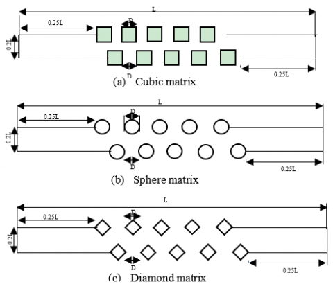
The flow was modelled using a representative unit of the matrix. Three matrix geometries were considered, the sphere, the cube and the diamond. The architecture and dimensions of the representative units are presented in Figure 2 and Table 1. The inlet and outlet space of length 0.25L were included to allow for flow development prior to entering the regenerator, to avoid back flow and allow for convergence of solution. Considering the size of the unit, a uniform mass flow and constant solid phase temperature assumptions were considered tenable. Also, translationally periodic boundary conditions were imposed at the inlet and outlet sections of the unit. A summary of the boundary conditions are shown in Table 2. Computational fluid dynamics code- ANSYS FLUENT was used for 2D simulation of the system with air as the working fluid. The properties of air used are presented in Table 3 and are assumed to be independent of temperature.
The maximum face size of mesh was set to 5e-06m after a grid sensitivity analysis and Inflation layers defined at the boundaries of the solid and continuum domain to enhance the accuracy of the result at the boundaries. Coupled scheme was used for pressure/velocity coupling and pseudo transient condition was imposed to enhance convergence. The system was considered as a steady state system and set to run for 500 iterations after hybrid initialization and patching of fluid domain at 306.5k.
Figure 2. Representative units of the regenerator matrix
Table 1. Parameters of the representative units
|
Geometry Parameter |
Sphere matrix |
Cubic matrix |
Diamond matrix |
|
Porosity $(\mathcal{E})$ |
0.813 |
0.751 |
0.8733 |
|
Area occupied by matrix (m2) |
3.74E-08 |
4.98E-08 |
2.53E-08 |
|
Perimeter of matrix (m) |
1.53E-03 |
2.00E-03 |
2.12E-03 |
|
Hydraulic diameter m |
4.24E-04 |
3.01E-04 |
3.29E-04 |
|
Mean flow area (m2) |
1.63E-07 |
1.50E-07 |
1.75E-07 |
|
D (m) |
1E-04 |
1E-04 |
1E-04 |
|
L (m) |
1E-03 |
1E-03 |
1E-03 |
Table 2. Boundary conditions
|
Region/ Boundary |
Condition |
|
Inlet/outlet |
Translational periodic |
|
Fluid/matrix boundaries |
Interface |
|
Top/bottom |
Symmetry |
|
Bulk fluid temperature |
Constant at 320K |
|
Matrix Wall temperature |
Constant at 293K |
|
Matrix surface |
No slip condition and stationary wall |
Table 3. Properties of air used for simulation
|
Air |
Properties |
|
density |
$1.225 k g / m^{3}$ |
|
Specific heat $\boldsymbol{C}_{\boldsymbol{v}}$ |
$718 J / k g K$ |
|
Thermal conductivity k |
0.0242 w/mK |
|
Viscosity |
1.7894e-05 Kg/ms |
The simulation results and computed parameters for the three geometries are presented in tables 4-9 and The effect of matrix geometry on flow and thermal dynamics of regenerators were discussed with respect to their behavior at low and high Re. For this study, the values of $R e \leq 25$ were considered as low, this is the range within which pressure drop with respect to velocity is linear therefore the flow is dominated by viscous forces. At Re>85 the inertial forces dominate and pressure drop with respect to velocity is quadratic.
Table 4. Data from spherical matrix simulation
|
$\boldsymbol{\dot{m}}_{f} \boldsymbol{k} \boldsymbol{g} \boldsymbol{S}^{-1}$ |
$u m S^{-1}$ |
Re |
$\boldsymbol{P}_{i n} \boldsymbol{N} \boldsymbol{m}^{-2}$ |
$\boldsymbol{P}_{\text {out }} \boldsymbol{N} \boldsymbol{m}^{-2}$ |
|
1.00E-07 |
0.000705 |
2.05E-02 |
0.00117 |
-0.0025 |
|
1.00E-06 |
0.00705 |
2.05E-01 |
0.0117 |
-0.025 |
|
1.00E-05 |
0.0705 |
2.05E+00 |
0.116 |
-0.25 |
|
1.00E-04 |
0.708 |
2.06E+01 |
1.185 |
-2.59 |
|
5.00E-04 |
3.640 |
1.06E+02 |
3.270 |
-3.75 |
|
8.00E-04 |
5.945 |
1.73E+02 |
7.470 |
-5.76 |
|
1.00E-03 |
7.514 |
2.18E+02 |
11.252 |
-7.01 |
|
2.00E-03 |
15.840 |
4.60E+02 |
40.920 |
-13.13 |
|
3.00E-03 |
24.143 |
7.01E+02 |
80.200 |
-19.39 |
|
4.00E-03 |
32.510 |
9.44E+02 |
121.740 |
-26.29 |
Table 5. Data from spherical matrix simulation
|
$\boldsymbol{T}_{\text {out}} \boldsymbol{K}$ |
$\boldsymbol{d} \boldsymbol{p} / \boldsymbol{L} \boldsymbol{N} \boldsymbol{m}^{-3}$ |
LMTD |
$\boldsymbol{h} \mathbf{W} \cdot \mathbf{m}^{-2} \cdot \mathbf{K}^{-1}$ |
$Q J$ |
|
309.09 |
3.67 |
21.076 |
1.41E+03 |
0.001 |
|
308.93 |
36.72 |
20.982 |
1.43E+04 |
0.011 |
|
308.83 |
366.20 |
20.920 |
1.45E+05 |
0.112 |
|
303.21 |
3775.12 |
17.267 |
2.64E+06 |
1.689 |
|
297.27 |
7015.01 |
12.324 |
2.51E+07 |
11.439 |
|
298.12 |
13230.00 |
13.158 |
3.62E+07 |
17.618 |
|
298.72 |
18258.00 |
13.7143 |
4.22E+07 |
21.415 |
|
301.40 |
54047.00 |
15.930 |
6.35E+07 |
37.439 |
|
302.93 |
99586.00 |
17.066 |
8.16E+07 |
51.537 |
|
303.85 |
148030.30 |
17.7147 |
9.92E+07 |
65.015 |
Table 6. Data from cubic matrix simulation
| $\boldsymbol{\dot{m}}_{f} \boldsymbol{k} \boldsymbol{g} \boldsymbol{S}^{-1}$ |
$u m S^{-1}$ |
Re |
$P_{i n} N m^{-2}$ |
$\boldsymbol{P}_{\text {out }} \boldsymbol{N} \boldsymbol{m}^{-2}$ |
|
1.00E-07 |
0.00097 |
2.00E-02 |
0.00242 |
-0.0034 |
|
1.00E-06 |
0.00967 |
1.99E-01 |
0.0242 |
-0.034 |
|
1.00E-05 |
0.0967 |
1.99E+00 |
0.243 |
-0.335 |
|
1.00E-04 |
0.967 |
1.99E+01 |
2.530 |
-3.268 |
|
5.00E-04 |
4.810 |
9.89E+01 |
18.340 |
-13.062 |
|
8.00E-04 |
7.680 |
1.58E+02 |
37.159 |
-17.120 |
|
1.00E-03 |
9.598 |
1.98E+02 |
52.914 |
-17.569 |
|
2.00E-03 |
19.540 |
4.03E+02 |
160.134 |
-4.379 |
|
3.00E-03 |
29.430 |
6.06E+02 |
279.810 |
29.566 |
|
4.00E-03 |
39.390 |
8.12E+02 |
403.182 |
84.981 |
Table 7. Data from cubic matrix simulation
|
$\boldsymbol{T}_{\text {out}} \boldsymbol{K}$ |
$d p / L N m^{-3}$ |
LMTD |
$\boldsymbol{h} \mathbf{W} \cdot \mathbf{m}^{-2} \cdot \mathbf{K}^{-1}$ |
$\boldsymbol{Q} \boldsymbol{J}$ |
|
310.06 |
5.82 |
21.651 |
9.28E+02 |
0.001 |
|
309.68 |
58.20 |
21.428 |
9.73E+03 |
0.010 |
|
309.48 |
578.01 |
21.311 |
9.97E+04 |
0.106 |
|
303.40 |
5798.00 |
17.399 |
1.93E+06 |
1.671 |
|
297.44 |
31402.00 |
12.497 |
1.82E+07 |
11.353 |
|
298.32 |
53927.00 |
13.347 |
2.63E+07 |
17.456 |
|
298.91 |
70483.20 |
13.882 |
3.07E+07 |
21.226 |
|
301.68 |
164513.00 |
16.145 |
4.59E+07 |
36.872 |
|
303.14 |
250243.70 |
17.216 |
5.94E+07 |
50.905 |
|
304.05 |
318201.30 |
17.856 |
7.22E+07 |
64.190 |
Table 8. Data from diamond matrix simulation
|
$\boldsymbol{\dot{m}}_{f} \boldsymbol{k} \boldsymbol{g} \boldsymbol{S}^{-1}$ |
$u m S^{-1}$ |
Re |
$P_{i n} N m^{-2}$ |
$\boldsymbol{P}_{\text {out }} \boldsymbol{N} \boldsymbol{m}^{-2}$ |
|
1.00E-07 |
0.000650 |
1.46E-02 |
0.00114 |
-0.0021 |
|
1.00E-06 |
0.00650 |
1.46E-01 |
0.0114 |
-0.0200 |
|
1.00E-05 |
0.0650 |
1.46E+00 |
0.112 |
-0.2000 |
|
1.00E-04 |
0.6650 |
1.50E+01 |
1.144 |
-2.2700 |
|
5.00E-04 |
3.800 |
8.56E+01 |
14.720 |
-12.101 |
|
8.00E-04 |
6.485 |
1.46E+02 |
38.465 |
-16.180 |
|
1.00E-03 |
8.33 |
1.88E+02 |
61.117 |
-16.700 |
|
2.00E-03 |
17.643 |
3.97E+02 |
242.633 |
0.464 |
|
3.00E-03 |
26.899 |
6.06E+02 |
498.000 |
34.470 |
|
4.00E-03 |
36.05 |
8.12E+02 |
786.810 |
74.600 |
Table 9. Data from diamond matrix simulation
|
$\boldsymbol{T}_{\text {out}} \boldsymbol{K}$ |
$d p / L N m^{-3}$ |
LMTD |
$\boldsymbol{Q} \boldsymbol{J}$ |
$\boldsymbol{Q} \boldsymbol{J}$ |
|
307.45 |
3.14 |
20.078 |
2.48E+03 |
0.0013 |
|
307.26 |
31.40 |
19.958 |
2.54E+04 |
0.0130 |
|
307.15 |
312.40 |
19.888 |
2.57E+05 |
0.1300 |
|
299.58 |
3414.00 |
14.462 |
5.61E+06 |
2.0550 |
|
296.80 |
26821.00 |
11.832 |
3.89E+07 |
11.6750 |
|
298.48 |
54644.95 |
13.494 |
5.07E+07 |
17.3270 |
|
299.54 |
77817.00 |
14.430 |
5.63E+07 |
20.5915 |
|
303.18 |
242169.00 |
17.244 |
7.75E+07 |
33.8563 |
|
304.92 |
463530.00 |
18.444 |
9.74E+07 |
45.5309 |
|
306.63 |
712210.00 |
19.559 |
1.09E+08 |
53.8239 |
4.1 Thermal analysis
The focus here was on the quantity of heat that the regenerators were able to extract from the hot fluid flowing through them and the dynamics that influenced it. Mass weighted average temperatures at exit of the regenerators $T_{\text {out}}$ were taken at 10 different values of Re. Mass averaged temperatures were used because the interest was on the variation of thermal energy of fluid mass as they flow through the system.
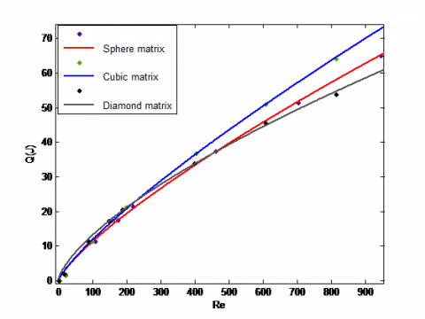
First the heat supply to the regenerator matrix(Q) by the working fluid was computed by balancing the energy of the fluid at inlet and exit using Eq. (2). The graphs of Q as a function of Re was shown in Figure 3 for the three geometries. From the figure, there was an increase in Q as Re increases due to improved fluid/matrix interaction arising from increase in turbulence and mass flow through the system.
Figure 3. Heat transfer to regenerator as a function of Re
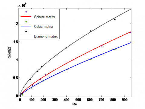
The area of matrix in contact with the fluid constitute the convective heat transfer surface and is a major determinant of heat transfer in the system. These surfaces are unequal for the three regenerator design. For an unbiased investigation of influence of matrix geometry on performance, heat transfer per unit area of matrix q was plotted in Figure 4.
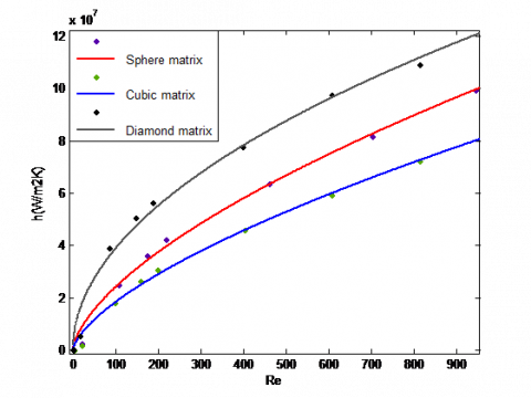
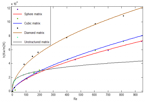
Diamond matrix design gave the best performance followed by sphere and cubic design respectively. A plot of convective heat transfer coefficient h as function of Re in Figure 5 also showed a similar trend.
Figure 4. Heat transfer/unit area of matrix with respect to Re
Figure 5. Convective heat transfer as a function of Re
4.2 Physics of heat transfer
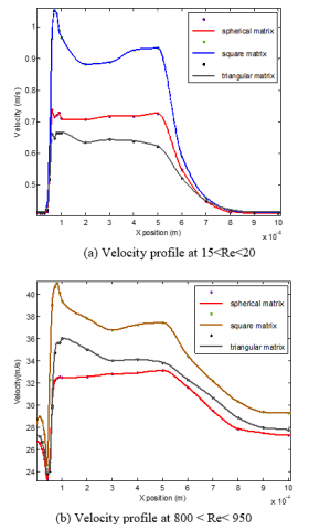
Convective heat transfer coefficient (h) is influenced by factors such as flow dynamics and thermal boundary layer thickness[18]. The graph of velocity across the length of representative unit of the regenerators in Figure 6a showed that for a given mass flow rate the velocity at inlet and through the regenerators correlate well with the mean flow area at low values of Re. The smaller the flow area, the higher the velocity. This is because of the attached and symmetric nature of the flow at this condition. At high Re (Figure 6b), there was a rapid rise in velocity of the diamond bed following the low flow resistance of streamlined edges of the matrix.
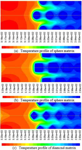
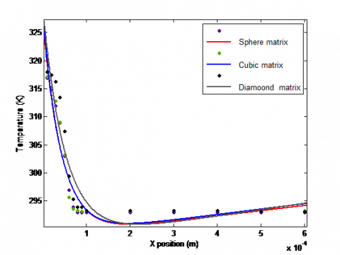
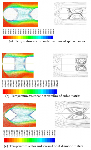
The static temperature profile downstream of the flow (Figure 7) and its plot with respect to position (Figure 8) at 15<Re<20 showed heat transfer from the fluid to the matrix is more rapid in cubic geometry, followed by sphere albeit slightly and then diamond. A trend that is consistent with area of the matrix in contact with the fluid. The smaller the area of convective heat transfer surface the longer it takes for for the fluid to exchange heat with the matrix.
At high values of Re, there was flow separation, which gave rise to low pressure and low velocity spinning vortex or eddies downstream of the matrix (Figure 9). The structure/size of the vortex and the point on the surface of the matrix where the flow separated varied with the geometry. The turbulence in a system is characterized by the vortex formation which consists of wide range of length and time scale. Large vortices draws its energy from the mean flow velocity and are responsible for mass and energy transport in the system. Large scale vortices are most prominent in diamond matrix design resulting in an increase in the convective heat transport. This is followed by sphere and cubic designs respectively.
Figure 6. Velocity profile across the length of the representative unit of the regenerators
The flow separation occurred at the face upstream of the matrix for cubic bed, at the vertices for the diamond and at an angle of about 80-85 degrees measured from the stagnation point for sphere. Thermal boundary layer which is inversely proportional to the heat transfer coefficient increases downstream of the matrix from the point of flow separation. Therefore this in addition to vortex formation explains the variations in the effectiveness of heat transfer for the three geometries.
Figure 7. Regenerator Static temperature profile at 15<Re<20
Figure 8. Static temperature plot with respect to position in the flow direction at 15<Re<20
Figure 9. Static temperature vector plot and streamline at 800<Re< 950
4.3 Pressure losses
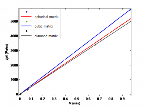
The pressures $P_{i n}$ and $P_{out}$ at inlet and exit of the regenerator (Table 4-Table 9) were computed using the area weighted average as that made the most physical sense. Velocity was computed as the bulk velocity at the minimum flow area using mass weighted average. Pressure loss ($d p / L$) across the regenerator matrix is governed by Eq. (11). At low Re, viscous forces dominates the system while inertial forces dominate at high Re thus the trivial terms can be neglected in turn [20, 23]. This then implies that at low values of Re, $d p / L$ is proportional to $\mu \mathbf{u}$ while at high Re it is proportional to $\frac{1}{2} \rho u^{2}$.
The plots of pressure drop with respect to velocity at low Re were shown in Figure 10. Relating the slope of the graphs to Darcy’s law Eq. (12) the permeability (k) for the three geometries were computed and presented in Table 10. k is proportional to the surface area of the matrix (Am) in contact with the fluid.
Table 10. Permeability of the geometries
|
Geometry |
Sphere |
Cube |
Diamond |
|
Permeability (m2) |
3.352e-09 |
2.983e-09 |
3.478e-09 |
Figure 10. Pressure drop with respect to velocity at low Re
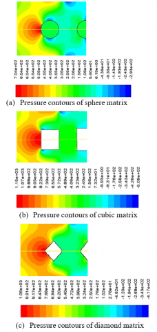
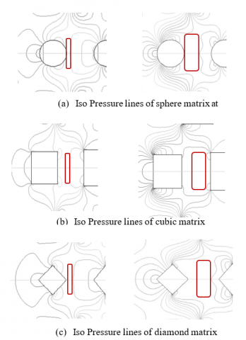
Figure 11. Pressure contours around the matrix at 800<Re<950
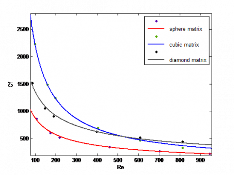
The pressure contours around the matrix at 800<Re<950 was shown in Figure 11. Pressure is maximum at the face of the matrix in contact with the fluid upstream of the flow. This sharp rise in pressure is known as adverse pressure gradient. This in addition to increase in inertial forces relative to viscous forces at high values of Re is what causes the flow to separate. From the point of separation, up to the face of the matrix downstream of the flow (wake), the pressure is constant and low relative to the corresponding region upstream. Using Eq. 13, the inertial resistance factors Cf at different values of Re was computed and plotted against Re in Figure 12. Cf decreased with increase in Re and can be used to describe the number of pressure heads over a given regenerator length [24]. A review of the values of Cf (Figure 12) and the pressure contours (Figure 13) shows that Cf is proportional to the cross-sectional area of the wake region.
Figure 12. Plot of inertial resistance factor Cf against their corresponding Re
Figure 13. Comparison of the size of wake at 80<Re<110 and 800<Re<950 respectively
For a regenerator, the most critical factors are the thermal effectiveness and pressure losses in the system [25]. Therefore, choosing a regenerator for a particular use involves a compromise between the two. The ratio $\mathrm{C}_{\mathrm{f}} / q$ was used to quantify this. A plot of this ratio with respect to Re (Figure 14) showed that sphere and diamond beds gave a similar and better performance than cubic beds.
Figure 14. A plot of the $\mathrm{C}_{\mathrm{f}} / q$ ratio with respect to Re
Figure 15. Comparison of convective heat transfer coefficient of matrix with defined geometry and unstructured matrix
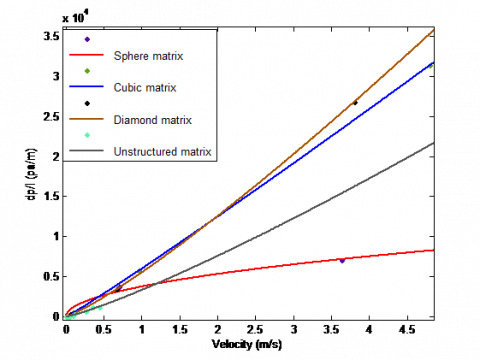
Figure 16. Comparison of pressure drops against velocity for matrix with defined geometry and unstructured matrix
4.4 Result comparison
The results of ANSYS CFX CFD simulation carried out by Jeremy [11] to determine the convective transport properties in porous material using unstructured matrix developed by Dyke were compared to those of the structured matrix above in Figure 15 and Figure 16.
It has been established that heat transfer in regenerators depend on the area of convective heat transfer surface and heat transfer coefficient of the system. Heat transfer coefficient depend majorly on the scale of the vortices developed and thermal boundary layer thickness both of which are greatly influenced by the geometry of the matrix. Large scale vortices draws from the mean flow velocity and are responsible for mass and energy transport within the system.
Thermal boundary layer thickness is inversely proportional to heat transfer coefficient and it increases downstream of the matrix from the point of flow separation which varried with geometry. This separation results from adverse pressure gradient at the face of the matrix in contact with the fluid upstream of the flow and increase in inertial forces relative to viscous forces at high Re. For cubic matrix it occurred at the face upstream of the flow, at the vertices for the diamond matrix and for the sphere the separation was at 80-85° from the surface measure from the stagnation point. The combined effect of vortex development and thermal boundary layer thickness places the diamond bed as most effective for heat convection. °
Pressure loses in the system are undesirable and was found to be a function of friction coefficient ($\mathrm{C}_{\mathrm{f}}$) which is proportional to the cross-sectional area of the wake region. The least pressure drop was recorded in sphere beds for all values of Re. The ratio $\mathrm{C}_{\mathrm{f}} / q$ was used as a measure of suitability of matrix geometry for use in a regenerator. Of the three, the sphere and diamond matrix gave a similar and better performance than the cube for all range of Re considered.
We wish to acknowledge the financial support from TETFUND IBR research grant.
A Area, m2
C Circumference of the matrix, m
Cf Inertial resistance factor
Cp Specific heat, J. kg-1. K-1
d Diameter, m
h Convective heat transfer coefficient, W.m-2
k permeability of matrix material
K Thermal conductivity, W.m-1. K-1
$\dot{\mathrm{m}}$ Mass flow rate, kg.S-1
L Length of regenerator, m
Nu Nusselt number
$p$ Pressure, Nm-2
Pr Prandtle number
Q Heat transfer, J
q Heat transfer per unit area, J.m-2
Re Reynolds number
T Temperature, K
t Time, S
u X component velocity, m.S-1
v Y component velocity, m.S-1
V Volume, m3
w Z component velocity, m.S-1
D Transverse dimension of matrix, m
L Length of regenerator, m
Greek symbols
$\mu$ Dynamic viscosity of air
$\rho$ Density
$\mathcal{E}$ Porosity
Subscripts
Conv Convection
m matrix
in Regenerator inlet
out Regenerator outlet
lm log mean
s supplied quantity
r rejected quantity
v constant volume (specific heat)
w matrix wall
p Spherical particle (diameter)
h hydraulic (diameter)
f Fluid (air)
wf matrix wall/fluid intersection
[1] Judkins, R.R., Fulkerson, W., Sanghvi, M.K. (1993). The dilemma of fossil fuel use and global climate change. Energy & Fuels, 7(1): 14-22. http://dx.doi.org/10.1080/02648725.2002.10648032
[2] Noel, N.P. (1986). Automotive Stirling Engine. Washington, D.C: U.S Department of Energy, Conservation and Renewable Energy.
[3] Gordon, R., Mayhew, Y. (2011). Engineering Thermodynamics Work and Heat Transfer (4th ed). New Delhi: Dorling Kindersley (India) Pvt. Ltd.
[4] Eastop, T., McConkey, A. (2003). Applied Thermodynamics for Engineering Technologist (5th ed.). Delhi: Pearson Education.
[5] Timothy, K.R. (1994). Composite matrix regenerator for stirling engines. Ohio: NASA Lewis Research Center.
[6] Faruoli, M., Viggiano, A., Magi, V. (2018). An investigation of thermo-fluid dynamic performance of a Stirling engine regenerator by means of OpenFOAM. Modelling. Measurement and Control B, 87(9): 151-158. https://doi.org/10.18280/mmc_b.870306
[7] Liu, Y. (2015). Dead volume effects in passive regeneration: Experimental and numerical characterization (Doctoral dissertation). University of Victoria, Victoria.
[8] Maria, F., Annarita, V., Vinicio, M. (2019). A porous media numerical approach for the simulation of stirling engine regenerators. Tecnica Italiana-Italian Journal of Engineering, LXIII(2-4): 291-296, https://doi.org/10.18280/ti-ijes.632-425
[9] Formosa, F., Despesse, G. (2010). Analytical model for Stirling cycle machine design. Energy Conversion and Management, 51(10): 1855-1863. http://dx.doi.org/10.1016/j.enconman.2010.02.010
[10] Aliabadi, A.A., Thomson, M.J., Wallace, J.S., Tzanetakis, T., Lamont, W., Di Carlo, J. (2009). Efficiency and emissions measurement of a Stirling-engine-based residential microcogeneration system run on diesel and biodiesel. Energy & Fuels, 23(2): 1032-1039. https://doi.org/10.1021/ef800778g
[11] Jeremy, V. (2017). Modelling of convective heat transfer in porous media. Ontario: University of Western Ontario. https://ir.lib.uwo.ca/etd/4852, accessed on Jul. 10, 2018.
[12] Kuldeep, P., Kesarwani, A. (2016). Unsteady CFD analysis of regenerator. International Journal of Scientific & Engineering Research, VII(12): 277-280.
[13] Falk, C. (2009). Predicting the performance of regenerative heat exchanger. Lund: 2009MVK160 Heat and Mass Transport.
[14] Michel, F.M., Sedat, T. (2009). Convective Heat Transfer. London: ISTE LTD & John Wiley and Sons Inc.
[15] Khan, W.A., Culham, J.R., Yovanovich, M.M. (2006). Convection heat transfer from tube banks in cross flow; analytical approach. International Journal of Heat and Mass Transfer, 49(25-26): 4831-4838, http://dx.doi.org/10.1016/j.ijheatmasstransfer.2006.05.042
[16] Baharami, M. (2018). Convection Heat Transfer. ENSC, 1-11. http://www.stu.ca/mbarami/ENSC%2520388/N, accessed on Aug. 20, 2018.
[17] Kamel, M.S. (2014). A numerical study of heat transfer and fluid flow in a bank of tubes with integral wake splitter. Journal Impact Factor, 5(12): 36-46.
[18] Adam, N., Dominique, D., Bert, B., Jan, C. (2006). CFD Calculation of Convective Heat Coefficients Validation-part 1 Laminar Flow. Annex 41–Kyoto, April 3rd to 5th.
[19] Andre, B. (2006). Applied Computational Fluid Dynamics. http://www.bakker.org, accessed on Sep. 21, 2018.
[20] Shankar, V., Bengtson, A., Fransson, V., Hagentoft, C.E. (2015). Influence of heat transfer processes in porous media with air cavity-A CFD analysis. In 8th International Conference on Computational and Experimental Methods in Multiphase and Complex Flow, Valencia, Spain, pp. 20-22. http://dx.doi.org/10.11159/ffhmt17.161
[21] Andersson, B., Andersson, R., Håkansson, L., Mortensen, M., Sudiyo, R., Van Wachem, B. (2011). Computational Fluid Dynamics for Engineers. Cambridge University Press.
[22] John, L.I., John, L.V. (2001). A Heat Transfer Textbook (3rd ed.). Cambridge, Massachussettes: John, Lienard, V.
[23] ANSYS, Inc. (2010). ANSYS Fluent User; Guide. Southpointe: ANSYS, Inc.
[24] Ruhlich, I., Quack, H. (2002). Investigations of regenerative heat exchanger. In Cryocoolers 10, 265-274. Springer, Boston, MA. http://dx.doi.org/10.1007/0-306-47090-X_31
[25] Chakrabarty, S.G., Wankhede, U.S. (2012). Flow and heat transfer behaviour across circular cylinder and tube banks with and without splitter plate. International Journal of Modern Engineering Research (IJMER), 2(4): 1529-1533.