Yuriy Bіlonoga* | Volodymyr Stybel | Oksana Maksysko | Uliana Drachuk
© 2020 IIETA. This article is published by IIETA and is licensed under the CC BY 4.0 license (http://creativecommons.org/licenses/by/4.0/).
OPEN ACCESS
This article analyzes the vast material of works devoted to the use of nanofluids in heat exchange equipment. It is proved that the use of the classical theories and equations for calculating the viscosities and thermal conductivities of nanofluids is not correct, since it does not coincide with the experimental results of most independent authors. A model of the chaotic motion of a nanoparticle is presented taking into account surface tension forces in a liquid coolant. The experimental results of the work of Malaysian and Iran authors on the effect of TiO2 nanoparticles with a concentration of 0.5%; 1.0% and 1.5% in the main liquid solution of ethylene glycol (EG) in water in a volume ratio of 40:60% in terms of heat transfer coefficient are compared with our theoretical studies. The results of the experiments presented in: an increase in heat transfer coefficients by 9.72%, 22.75%, 28.92% for 1.5% volume concentration of TiO2 nanoparticles at a coolant temperature of 30℃, 50℃, 70℃, respectively. Our theoretical result: increase in the obtained heat transfer coefficients by 9.79%, 22.22%, 29.09% according to our formulas (9, 10, 15) for calculating turbulent viscosities and thermal conductivities, which takes into account the effect of surface tension forces on the total flow of nanofluids in the channels of heat exchange equipment. A new method for calculating heat exchange equipment using nanofluids is presented, taking into account the action of surface tension forces, as well as predetermining the calculation of turbulent viscosities and thermal conductivity of nanofluids. A theoretical calculations a plate heat exchangers for a technological task performed by classical and new method is presented. Similar results were obtained, which differ by about 0.5 of a percent. The plate heat exchanger was calculated using a new method using TiO2 nanoparticles in water and in a mixture of EG in water in a ratio of 40:60%, as well as when pumpkin vegetable oil was added to milk with the optimal concentration.
nanofluids, heat exchange equipment, viscosity turbulent, thermal conductivity turbulent, surface tension coefficient
Today, the lion's share of energy losses in the food, processing, pharmaceutical industry occurs when using heat exchange equipment. The relatively low energy efficiency of heat exchange processes allows scientists to propose various methods for reducing heat losses in heat transfer systems.
So, to improve the heat transfer coefficients of pipe heat exchangers, the authors propose to use spiral-shaped inserts, contributing to the intensification of the turbulization of the liquid flow of heat transfer media [1-3]. However, this method has several drawbacks:
- an increase in the overall hydraulic resistance of the system, which may to level the increase in thermal efficiency;
- the complexity of cleaning pipes with spiral inserts from contamination;
- a significant increase in metal intensity and cost of such heat exchangers, especially with the use of copper inserts.
It should be noted that the choice and the theoretical calculation of heat exchangers with spiral inserts is significantly complicated as the structure of the criterion equations using Nusselt numbers varies depending on the material and geometry of the inserts, as well as other regime heat transfer parameters.
In order to increase the heat transfer of various heat exchange systems, spiral corrugated pipes are also proposed [4, 5]. However, this method also has a number of drawbacks:
- a similar increase in the total hydraulic resistance;
- the complexity of cleaning the pipes from contamination;
- a significant complication and an increase in the technology of manufacturing such spiral corrugated pipes.
To eliminate the above disadvantages, as well as to improve the efficiency of heat exchangers in the liquid-liquid system, various additives to heat transfer fluids are used today. These additives are aimed at improving their heat-exchange properties and frost resistance, as well as increasing the boiling point of fluid in automotive radiators. These include ethylene, – propylene and di-propylene glycols of various concentrations in water. Also, nanofluids are widely used to increase the efficiency of heat exchange apparatuses as additives to heat carriers [6, 7]. Some scientific works are devoted to mating combinations of various methods of enhancing heat transfer in heat exchangers, for example, using nanofluids simultaneously with spiral twists [8, 9], using nanopowders with ethylene or propylene glycol additives to water [10].
Improving the heat transfer properties of liquids using these methods is not in any doubt. These are very promising areas of research. However, works on enhancing the heat transfer properties of liquids using nanoparticles is very controversial [11].
Thus, in the works [12-15], it was shown that the increase in heat transfer when using nanofluids is anomalously high and is not described by known equations.
Thus, it was stated in the work [12] that the improvement in heat transfer properties containing 0.5 wt.%. Nanoparticles reaches more than 350% at Re = 800, which cannot be explained only by the high thermal conductivity of nanofluids.
In the work [13], the maximum heat transfer coefficient enhancement is 104%.
In the work [14], anomalously high thermal conductivity coefficient was observed when using nanotubes in an oil medium, indicating the impossibility of using traditional thermal conductivity models for solid - liquid suspensions.
In the works [16-20], on the contrary, it was shown that the experimental results correlate well with the theoretical ones.
In the work [16], it was shown that the heat transfer coefficient and the friction coefficient of TiO2-water nanofluids (21 nm in diameter, dispersed in water with a volume concentration of 0.2 – 2%) in a horizontal two-pipe countercurrent the heat exchanger under turbulent flow conditions was about 26% larger than that of pure water.
In the work [17], nanofluids with an average particle size of 50 nm and 22 nm, respectively, are used. Increasing the viscosity and thermal conductivity of TiO2 gives the maximum increase in heat transfer by 26%.
The effect of temperature on heat transfer using TiO2 nanofluid with a Reynolds number Re =25000 and TiO2 concentrations of 0.5%, 1.0% and 1.5% was studied in [19]. The base fluid used was a mixture of distilled water and ethylene glycol (EG) in a volume ratio of 60:40. At 30℃ and at a volume concentration of 1.5%, the increase in the heat transfer coefficient was 9.72%. An increase of 22.75% and 28.92% was at 50℃ and 70℃, respectively.
In work [20], four volume concentrations of nanofluids (1%, 2%, 3% and 4%) were used; It has been established that TiO2 nanofluid increases the efficiency of heat transfer by up to 20% compared to pure water.
For works [16-20], it is analogous that TiO2 with concentrations of about 1.5% was used as nanoparticles and maximum increase in the heat transfer coefficient was observed at about (20-30) %.
However, the theoretical calculation, selection and optimization of heat exchangers when using nanofluids encounters serious difficulties in terms of classical approaches using numerical equations and Nusselt numbers. This is due to the fact that when using nanofluids in heat exchangers, classical equations do not work, because they are not sensitive to additives to liquids at the nano level within no more than 5%. As a result, experimenters record a significant improvement in the heat transfer properties of liquids with nanoparticles, the theoretical calculation of such heat exchangers using nanofluids is difficult. Dispersity, material, concentration and other parameters of nanoparticles affect the shape and structure of numerical equations, and when using specific nanofluids, it is necessary to derive the corresponding empirical numerical equation, which requires many time-consuming experiments.
Quite a lot of work has been devoted to studying the effect of changes in the thermal characteristics of coolants when exposed to nanoparticles of various concentrations [21-24]. Such characteristics, first of all, include viscosity, density, thermal conductivity and specific heat capacity when using nanofluids. All the mentioned characteristics of nanofluids are included in the numbers of Nusselt, Prandl and others, who take part in the, numerical, and exponential equations in the calculation and selection of optimal heat exchangers.
Due to the fact that many researchers are talking about more complex heat transfer mechanisms in nanofluids than in Newtonian ones, we are confident that the problems of heat transfer in such nanosystems should be considered taking into account surface forces. However, some authors propose to use surface tension coefficients and wetting angles when studying the behavior of nanofluids under heat transfer conditions [25-27]. However, these surface characteristics are not included in the numerical equations and do not take part in the classical calculations of heat exchangers using nanofluids, and therefore, in our opinion, these studies are purely experimental, empirical, but not systemic.
In the paper [28], which, in our opinion, carries a global approach to the study of the behavior of nanofluids in various heat exchange systems, important general conclusions were made:
- nanofluids should be considered as homogeneous, homogeneous Newtonian fluids;
- an increase in heat transfer coefficients when using nanofluids is equal to an increase in their thermal conductivities compared to the base fluid.
- heat-efficient nanofluid should have the highest possible thermal conductivity and the lowest possible viscosity.
However, this very thorough and necessary study, which was conducted by five independent groups of authors from various European countries and the USA, also used the classical approach to determining the overall heat transfer coefficients of heat exchangers using the Nusselt, Reynolds, Prandtl and other numbers. This approach is correct, but it is empirical and is based on the use of experimental numerical equations, in which the Nusselt number depends on many factors of the heat exchange system and is calculated by empirical exponential equations. The very important second and third conclusions of work [28] suggest the need for maximum thermal conductivity of nanofluids with minimal viscosity. However, the thermal conductivity and viscosity of nanofluids in this work is considered and determined under static conditions, and in heat exchange equipment turbulent flow of heat transfer media always prevail, where the turbulent viscosity and thermal conductivity of liquids are tens and hundreds of times higher than their tabular (classical), molecular values.
These features do not diminish the results of research by individual authors, however, we offer a slightly different approach to the systemic study of the behavior of nanofluids in heat exchange equipment, which is based on taking into account the influence of surface forces arising between nanoparticles and the base fluid, as well as at the interface between the metal wall and the liquid coolant.
The overwhelming majority of authors state a fairly significant increase in the overall heat transfer coefficients in heat exchange equipment using nanoparticles of various concentrations and dispersions. However, they speak of a significant difference between the calculated and experimental data on this issue and a possible more complex mechanism of heat exchange in nanofluids.
Based on our works [29-34], we concluded that our proposed model of contacting metal surfaces with regard to their the binding energy and surface energy [29-31], as well as consideration of the movement of heat-transfer fluids near the metal walls of the heat exchange equipment with taking into account surface forces [32-34], has the right to exist. Based on this, we set ourselves the following tasks in this work:
- choose from literature sources and analyze the numerical equations by which convection coefficients can be calculated, that is, by which the optimal heat exchange equipment can be calculated and selected when using nanofluids, for example, with TiO2 nanoparticles;
- show the consistency of the experimental data of a number of authors on increasing heat transfer coefficients when using nanofluids in heat exchangers with calculated data based on the use of classical numerical equations using the Nusselt Reynolds and Prandtl numbers;
- show the possibility of calculating shell-and-tube, plate and other types of heat exchangers taking into account the turbulent viscosity and thermal conductivity, as well as the specific heat capacity and the surface tension coefficient of the heat-transfer fluid with nanoparticles;
- show the full compliance of the new method of calculating heat exchange equipment, based on the use of the values of turbulent viscosities and thermal conductivities, as well as the usual and turbulent numbers Bl using nanofluids with experimental data from a number of independent authors.
3.1 Analysis of the forces acting on the nanoparticle, based on hydrodynamic similarity
In the work [35] it is indicated that the force acting on a nanoparticle that moves in a liquid is non-stationary, and therefore the application of the laws of hydromechanics to nanoparticles is not possible. The average diameter of small nanoparticles is actually commensurate with the size of the molecules of the base fluid, and therefore this statement is quite acceptable and justified. However, in this work we attempted to circumvent these warnings, using the concept of turbulent viscosity and thermal conductivity of liquid coolants, which we followed in the calculation and selection of heat exchangers in the works [33, 34].
When analyzing the forces acting on the nanoparticle itself, based on the similarity theory, we neglected the forces of gravity, Archimedes and inertia, since the average diameter of the nanoparticles is very small, and we took into account the force of surface tension and friction. In the Stokes formula, we enter the value of the turbulent viscosity. We also take into account the hydrophilicity of the wetting surface, which varies with the wetting angle at a certain point in time when the nanoparticle interacts with the base fluid at the molecular level. Since the action of surface tension forces is of a molecular nature [36], we consider such an approach quite acceptable.
Based on the above analysis, we write the equation, taking into account the surface tension force and friction force acting on the nanoparticle in the flow of a liquid heat carrier moving turbulently (1):
$\pi d\sigma \cos \theta =3\pi dV{{\mu }_{turb}}$ (1)
Based on our works [32-34], having written the value of turbulent viscosity in the central part of the coolant flow, we obtain (2):
$\sigma \cdot \cos \theta =\left( 3\cdot V\cdot B{{l}_{turb.}}\frac{\sigma \cdot \cos \theta }{\sqrt{{{C}_{p}}\cdot {{1}^{0}}K}} \right)$;
$B{{l}_{turb.}}=\left( \frac{\sqrt{{{C}_{p}}\cdot {{1}^{0}}K}}{3\cdot V} \right)$; (2)
At the same time, the value $\sqrt{{{C}_{P}}\cdot {{1}^{0}}K}$ reflects the speed of thermal movement at the molecular level, having the dimension m/s, and the value V is the linear speed of movement of the coolant with the nanoparticles at T mode. We also remind that the transitional viscosity of a fluid, the value of which we derived in previous works [33, 34], is the viscosity at the interface of LBL and turbulent flow, having dimension (Pa.s) and calculated by formula (3), and dimensionless turbulent number is the ratio of turbulent to transition viscosity (4) In addition, the dimensionless number Bl is (5) [33, 34].
${{\mu }_{trans.}}=\frac{\sigma \cdot \cos \theta }{\sqrt{{{C}_{p}}\cdot {{1}^{0}}K}}$ (3)
$B{{l}_{turb}}=\frac{{{\mu }_{turb.}}\cdot \sqrt{{{C}_{p}}\cdot {{1}^{0}}K}}{\sigma \cdot \cos \theta }$ (4)
$Bl=\frac{\mu \sqrt{{{C}_{p}}\cdot {{1}^{0}}K}}{\sigma \cdot \cos \theta }$ (5)
In particular, in the work [34], we presented the final formula for calculating the turbulent number Blturb. which has the form (6):
$B{{l}_{turb.}}={{\left( \frac{\sqrt{{{C}_{p}}\cdot {{1}^{0}}K}}{V} \right)}^{-X}}$ or $B{{l}_{turb.}}_{.}=\frac{1}{Bl}{{\left( \frac{\sqrt{{{C}_{p}}\cdot {{1}^{0}}K}}{V} \right)}^{-X}}\frac{\mu {{\sqrt{{{C}_{p}}\cdot {{1}^{0}}K}}_{.}}}{\sigma \cdot \cos \theta };$ (6)
In the Blturb. number we have derived, we compare turbulent viscosity and transitional viscosity (3). The transitional viscosity of the coolant is substantially higher than the molecular viscosity [33, 34]. If we want to compare the turbulent and molecular viscosity, then it must be borne in mind that, in the LBL itself, the viscosity of the fluid decreases from the transitive viscosity to the molecular viscosity. We introduce one more parameter – the transitional number Bltrans, which is the ratio of the transitional viscosity in the transitional zone LBL to the molecular viscosity of the heat-transfer fluid (7):
$B{{l}_{trans.}}_{.}=\frac{{{\mu }_{trans.}}}{\mu }=\frac{\sigma \cdot \cos {{\theta }_{.}}}{\mu \sqrt{{{C}_{p}}\cdot {{1}^{0}}K}}=\frac{1}{Bl};$ (7)
When comparing the turbulent viscosity of a liquid coolant with a molecular viscosity, we obtain the relation (8):
$\frac{{{\mu }_{turb.}}}{\mu }=B{{l}_{turb}}_{.}\cdot Bl;$ (8)
Or the final formula for calculating the turbulent viscosity of the coolant, taking into account the formula (6), is written in the form (9):
$\frac{{{\mu }_{turb.}}}{\mu }={{\left( \frac{\sqrt{{{C}_{p}}\cdot {{1}^{0}}K}}{V} \right)}^{-X}}\cdot Bl\,;$ ${{\mu }_{turb.}}=\mu \cdot {{\left( \frac{\sqrt{{{C}_{p}}\cdot {{1}^{0}}K}}{V} \right)}^{-X}}\cdot Bl;$ (9)
As a result, we obtained Eq. (9) for calculating turbulent viscosity, in which the dimensionless complex (turbulent number Blturb. is responsible for the turbulent, convective component of the coolant flow, and Bl for the molecular, static component. In this case, the turbulent thermal conductivity of the coolant will be calculated by the formula (10), and the heat transfer coefficient - by the formula (11). (where dЕis the equivalent diameter of the coolant flow).
${{k}_{turb.}}={{\mu }_{turb.}}\cdot {{C}_{P}};$ (10)
${{h}_{turb}}_{.}=\frac{{{k}_{t}}_{urb.}}{{{d}_{}}}$ (11)
As a comparison, we also present formula (12) for calculating the turbulent viscosity of air flows [33, 34, 37].
${{\mu }_{turb.}}=\frac{\mu \cdot a\sqrt{2\operatorname{Re}}}{0.769}$ (12)
From the formula (8) it is seen that the ratio of turbulent and molecular viscosity is the ratio $\left( \frac{B{{l}_{t}}_{urb.}}{Bl} \right)$. Comparing Eqns. (8), (6) and (2), we obtain Eq. (13):
${{\left( \frac{\sqrt{{{C}_{p}}\cdot {{1}^{0}}K}}{3\cdot V} \right)}^{0.5\div 1}}={{\left( \frac{\sqrt{{{C}_{p}}\cdot {{1}^{0}}K}}{V} \right)}^{-X}}\cdot B{{l}^{1\div 2}}$ (13)
The terms of relation (13) do not have stationary exponents and lie in the ranges indicated in (13), which can constantly change in these ranges at certain points in time due to the instability of the surface tension force acting on the nanoparticle.
Based on the foregoing, we propose to equate formulas (9 and 12) with each other in order to be able to obtain the value of degree X in a more convenient way and to obtain the relation (14):
$\frac{\mu \cdot a\sqrt{2\operatorname{Re}}}{0,769}=\mu \cdot {{\left( \frac{\sqrt{{{C}_{p}}\cdot {{1}^{0}}K}}{V} \right)}^{-X}}\cdot Bl$ (14)
Performing simple mathematical transformations and taking the logarithm, we obtain a new averaged, universal, empirical-analytical formula for calculating the degree of turbulization of the coolant flow X (15):
$-X=\frac{\ln \frac{a\cdot \sqrt{2\operatorname{Re}}}{0.769\cdot Bl}}{\ln \frac{\sqrt{{{C}_{p}}\cdot {{1}^{0}}K}}{V}}$ (15)
The formula (9) that we derived are actually universal numerical dimensionless equations for calculating heat exchange equipment, where the usual Reynolds and Prandtl numbers in fractional powers found empirically are not present.
In formula (9), the only turbulent number Blturb. is in the fractional degree X, whose value can be found analytically using the logarithmic relation (15). The degree of X depends on many factors, mainly related to the temperature of the coolant and the percentage ratio of nanoparticles in the liquid.
The optimization of the parameters of the functions, which is described by formulas (9-15), was carried out by us on a personal computer using the Mathcad software package.
The results of these numerical calculations of computer simulation are listed in Table 2 (A, B, C) (Appendix).
3.2 Comparison of experimental and calculated data of on the increase of heat transfer coefficients when using nanofluids TiO2
To test the efficiency of formulas (9, 10, 15) and compare ites with other numerical equations аs an example, we chose EG with the addition of TiO2 nanoparticles with an average diameter d = 50 nm. The most commonly used classical numerical equations for determining convection coefficients, including when using nanofluids with TiO2, in a turbulent flow regime look like this (Table 1).
In the work [19], an experimental material is presented on the values of thermophysical quantities for mixture of distilled water and EG in a volume ratio of 60:40 (Table 2(A), appendix).
The Table 2 is divided into three parts horizontally depending on the temperature of experiments 30; 50; 70℃ and into three parts vertically (A, B, C), where in (A) the experimental data from work [19] are presented, in (B) – our theoretical calculations of heat transfer coefficients according to the well-known Eqns. (15-20) [38-43] and in (C) – our theoretical calculations of turbulent viscosities and thermal conductivities according to our formulas (9, 10, 15).
Using the experimental results of the work [19], we calculated for all temperatures and thermo-physical quantities the values of turbulent viscosities and thermal conductivities using the formula (9) we derived. The hydrophilicity of the surfaces were chosen taking into account the work [25]. The surface tension coefficients of EG of the corresponding concentrations in water at appropriate temperatures were selected from the reference book [44].
In the calculations, within each temperature, for the possibility of fixing the percentage increase in the heat transfer coefficients, the Reynolds number was constant and equal to Re30 = 11.000, Re50 = 17.000 and Re70 = 22.000, respectively. These values of Reynolds numbers can be clearly seen in graphs (a), (b), (c) (Figure 3), [19].
As a result of a computer experiment using the program package Mathcad, the exponent X (degree of turbulization of the coolant flow) were obtained for temperatures of 30, 50 and 70℃, respectively: X30= 0.253; X50= 0.547; X70= 0.708 (Table 2 (C), appendix).
Table 2 (Appendix, columns 7–12) shows that a very positive experimental result obtained by the authors of [19] cannot be theoretically calculated using Eqns. (15–20, Table 1). At a temperature of 30℃, experiments and theoretical calculations differ little by 2–3%, with the exception of equation (20). However, at a temperature of 50℃ and especially 70℃, the difference in results is very noticeable. This is about 10% or more.
Table 1. Convective heat transfer correlations of TiO2 nanofluids
|
Numerical equation |
Relevant information |
|
$Nu=0.021\cdot {{\operatorname{Re}}^{0.8}}\cdot {{\Pr }^{0.5}}$ (15) [38] |
Experimental study Turbulent flow Al2O3/water nanofluids; TiO2/water nanofluids: $\begin{align} & (0.0\le \phi \le 3.0); \\ & ({{10}^{4}}\le \operatorname{Re}\le {{10}^{5}}); \\ & (6.5\le \Pr \le 12.3); \\ \end{align}$ |
|
$Nu=0.067\cdot {{\operatorname{Re}}^{0.71}}\cdot {{\Pr }^{0.35}}+0.00050\operatorname{Re}$ (16) [39] |
Experimental study Turbulent flow TiO2/water nanofluids: $\begin{align} & (0.2\le \phi \le 0.25\text{ }); \\ & (5\cdot {{10}^{3}}\le \operatorname{Re}\le 3\cdot {{10}^{4}}); \\ \end{align}$ |
|
$Nu=0.074\cdot {{\operatorname{Re}}^{0.707}}{{\Pr }^{0.385}}\cdot {{\varphi }^{0.074}}$ (17) [40] |
Experimental study Turbulent flow TiO2/water nanofluids $\begin{align} & (0.2\le \phi \le 2.0); \\ & (3\cdot {{10}^{3}}\le \operatorname{Re}\le 1.8\cdot {{10}^{4}}); \\ \end{align}$ |
|
$Nu=\frac{\text{(0}\text{.125}f\text{)(Re}-\text{1000)Pr}}{1+12.7{{(0.125f)}^{0.5}}\left( {{\Pr }^{2/3}}-1 \right)}$ (18) $f={{\left( 0.79\ln \operatorname{Re}-1.64 \right)}^{-2}}$ [41] |
Numerical study Fully developed turbulent flow: $\begin{align} & (3\cdot {{10}^{3}}\le \operatorname{Re}\le 5\cdot {{10}^{6}}); \\ & (0.5\le \Pr \le 2000); \\ \end{align}$ |
|
$Nu=\frac{\text{(0}\text{.125}f\text{)Re}\cdot \text{Pr}}{1.07+12.7{{(0.125f)}^{0.5}}\left( {{\Pr }^{2/3}}-1 \right)}$ (19) $f={{\left( 0.79\ln \operatorname{Re}-1.64 \right)}^{-2}}$ [42] |
Numerical study Fully developed turbulent flow: $\begin{align} & (5\cdot {{10}^{5}}\le \operatorname{Re}\le 5\cdot {{10}^{6}}); \\ & (0.5\le \Pr \le 2000); \\ \end{align}$ |
|
$N{{u}_{nf}}=0.0059(1+7.6286{{\varphi }^{0.6886}}Pe_{d}^{0.001})\operatorname{Re}_{nf}^{0.9238}\Pr _{nf}^{0.4}$ (20) [43] |
$\phi $– volume concentration (%) $\varphi $– volume fraction, $\phi =\frac{\varphi }{100}$; |
Сomparison with the experimental results of the base liquid without nanoparticles and with them at the indicated concentrations (indicated in bold in the Table 2, appendix) does not confirm a positive result for a 1.5% concentrations of 9.72% (30℃) and 22.75% (50℃) and 28.92% (70℃). In addition, the classical formulas and models for calculating the viscosities and thermal conductivities of nanosuspensions are also not suitable for calculating the viscosities and thermal conductivities of nanofluids. The paradox of this approach is that the classical equations for calculating heat exchange equipment (15–20, Table 1) contain the values of viscosity and thermal conductivity under conditions of a static coolant. The main inaccuracy of this approach, in our opinion, is that the amount of heat that is additionally transferred by chaotic moving nanoparticles in the turbulent heat carrier flow is not displayed or is barely displayed in the, molecular values of thermal conductivity and viscosity in static.
To eliminate such shortcomings, this article proposes an approach to studying the behavior of nanoparticles in turbulent coolant flows, taking into account surface forces.
As can be seen from the table 2(C) (columns 20 and 21), the increase in turbulent viscosity and thermal conductivity under the influence of TiO2 nanoparticles, calculated theoretically by us using the formulas (9, 10, 15), fully correlates with the experimental results of the work [19]. The discrepancy is observed at the level of up to 1%, which lies within the statistical errors of the experimental data and the operability of the formulas (9, 10, 15).
The turbulent viscosity and thermal conductivity, which we calculated using formulas (12 and 10), correlate with the experiments of work [19] much worse, but better than equations (15–20, Table 2(B), columns 13 and 14).
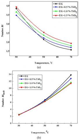
In the graphs, we presented the dependence of numbers Bl and Blturb. from temperature and the concentration of nanoparticles TiO2 in the base fluid. (Figure 1 a, b).
From Figure 1 (a) and (b) and Table 2 it can be seen that at a temperature of 30℃ the molecular Bl number is almost 1.5 times higher than turbulent number Blturb. This suggests that at relatively low temperatures, liquids with high molecular viscosity (type EG) cannot achieve high turbulent viscosity. With increasing temperature, the molecular viscosity decreases sharply and this makes it possible to sharply increase the degree X of turbulization of the flow. At 50℃, the number Bl of is already about 3 times less than the Blturb. number, and at 70℃ it is about 6-9 times less. (Table 2, C), columns 18, 19 are grayed out).
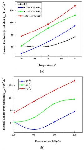
The dependence of the numbers Bl (a) and Blturb.(b) from the concentration of TiO2 in the nanofluid is shown in Figure 2. It can be seen from Figure 2 that the Blturb. number depends very little on concentration, since 1.5% of the maximum concentration weakly affects the degree of turbulization of the coolant flow. The concentration of particles in the base fluid affects the molecular Bl number is much more noticeable. And as a result: the turbulent thermal conductivity of the nanofluid increases from in temperature and in the concentration of the nanofluid (Figure 3). This explains the fact that nanoparticles transfer an additional part of thermal energy, and classical numerical equations, for example (15-20), do not record this. The formulas (9, 10, 15) that we derived are actually universal numerical dimensionless equations for calculating heat exchange equipment, where the usual Reynolds and Prandtl numbers in fractional powers found empirically are not present.
Figure 1. Dependences of numbers Bl (a) and Blturb. (b) on the temperature of the coolant
Figure 2. The dependence of the numbers Bl (a) and Blturb. (b) the concentration of nanofluid TiO2
Figure 3. Dependence of turbulent thermal conductivity on temperature (a) and concentration TiO2 (b) of the coolant
In formulas (9, 10), the only turbulent number Bl turb. is in the fractional degree X, whose value can be found analytically using the logarithmic relation (15). The degree of X depends on many factors, mainly related to the temperature of the coolant and the percentage ratio of nanoparticles in the liquid.
Our theoretical calculations, taking into account surface forces, were used in the work [45] to optimize openings in seeders while stabilizing seed planting.
It should be emphasized that the classical approach to the calculation of heat exchange equipment is based on the that the Nusselt number is calculated using numerical equations that depend mainly on the Reynolds and Prandtl numbers, where the Reynolds number has the maximum degree, i.e. the of the turbulent component is maximal (for example, Eqns. 15-20, Table 1). When nanoparticles are added to the base fluid, they always contribute to an increase in molecular viscosity (Table 2, A column 5), i.e. a decrease in the Reynolds number, since the molecular viscosity is in the denominator. In this case, the Prandtl number is almost unchanged, since the molecular viscosity and thermal conductivity, which are in the numerator and denominator, are mutually compensated. As a result, the heat transfer coefficient, using the classical equations, does not increase as much as in reality in the experiment. Therefore, a group of authors led by Rudyak in his works, for example, in the study [46], repeatedly indicates the impossibility of using classical equations for calculating heat transfer in nanofluids.
The classical approach works as long as the molecular thermal conductivity increases faster than the molecular viscosity. Consequently, the classical equations more or less correctly fix the increase in convection coefficients only at low temperatures. At high temperatures, the contribution of the turbulent component increases, and the classical equations do not work completely. The main inaccuracy of the classical approach, in our opinion, is that in the classical equations there are only molecular characteristics of the coolant flow (viscosity and thermal conductivity), and all heat transfer equipment is calculated on the basis of operation in turbulent conditions. In addition, surface forces are not taken into account.
Our approach to the calculation of heat exchange equipment is based on the account of the action of surface tension forces and turbulent viscosities as well as turbulent thermal conductivities of heat flows and is described by Eqns. (9, 10 or 12, 10). Looking at Eq. (9), we can see that the turbulent viscosity of the coolant is proportional to molecular viscosity, numbers Bl and Blturb. The Bl number is responsible for the molecular component, and the Blturb. number is responsible for the convective (turbulent) component.
Adding nanoparticles to the coolant has a positive effect if the product of the numbers Bl, Blturb. increasing. Under certain conditions, when the percentage of nanoparticles in the liquid becomes higher than a certain optimal value, the molecular component begins to prevail over the convective and the product of the numbers Bl, Blturb. may decrease. In this case, the indicator X, which is responsible for the degree of turbulization of the coolant flow at a certain maximum value of the number, can decrease. This clearly fixes in the formula (15). This explains the fact that most researchers say that the maximum concentration of nanoparticles in the base fluid should not exceed about 5% when the molecular component of the flow begins to slow its turbulence.
Our theoretical studies also correlate well with the results of work [47], where experimental material is presented on the effect of ТiО2 nanoparticles at concentrations of 0.24; 0.60; 1.18% vol. % on the base coolant – water. The behavior of L-and T-flow regimes of the coolant is investigated. Experiments have shown an increase in heat transfer coefficients of 4.63; 11.47 and 20.20% with coolant supply mode L and 4.04; 10.33 and 21.87% for flow regime T, respectively.
The product of the turbulent viscosity and heat capacity of the coolant gives turbulent thermal conductivity, and the heat transfer coefficient also includes a linear factor - the equivalent flow diameter or radius.
3.3 An example of the calculation of the plate heat exchanger according to the classical method
For a technological task, namely, heating cold milk with hot water, which was described in our previous works [33, 34], we calculated a shell-and-tube heat exchanger using a classical and new method. In this paper, we give an example of calculating the plate heat exchanger by the classical and new method for a similar technological problem.
1. Thermal and physical properties of milk and water for average temperatures [33, 34]:
- average temperature of cold milk Tc = 42.5℃;
- average temperature of hot water Th = 72.5℃;
- cold milk: ρc = 1020 kg.m-3; µc = 0.96·10-3 kg.m-1. s-1;
kc = 56.98·10-2 W.m-1. K-1; σc = 47.75·10-3 N.m-1;
cpc = 3.914·103 J.kg-1.K-1.
- hot water: ρh = 970 kg.m-3; µh = 0.41·10-3 kg.m-1. s-1;
kh = 67.7·10-2 W.m-1. K-1; σh = 62.25·10-3 N.m-1;
Сh = 4.198·103 J.kg-1.K-1;
2. The approximate surface area of heat transfer and the approximate overall heat transfer coefficient [33, 34]:
${{U}_{app}}\approx 800\text{ }W.{{m}^{-2}}.{{K}^{-1}}\text{ }{{A}_{app}}=\frac{Q}{\Delta {{T}_{LMTD}}{{U}_{app}}}=\frac{2113560}{28\cdot 800}=94\text{ }{{m}^{2}}$
From Table 2.13 [48], we choose a set of plates of a plate heat exchanger with an approximate heat transfer surface area calculated in paragraph 6 for a shell-and-tube heat exchanger [33, 34], that is, about 94 m2. Plate type – A= 0.6 m2; Number of plates – N = 170; Total area of the plates –
А = 100 m2; (this is the closest value to the approximate area Аapp = 94 m2 ).
3. The layout of the plates is the simplest C: 85/85 (N/2);
4. Cross section between the plates [48, p. 63] –
Across. = 0.00245 m2;
5. The rate Across of movement of cold milk between the plates
${{V}_{c}}=\frac{{{m}_{c}}}{{{\rho }_{c}}N\cdot {{A}_{cross}}}=\frac{12}{1020\cdot 85\cdot 0.00245}\text{ }=\text{ }0.0565\text{ }m.{{s}^{-1}};$
6. The equivalent diameter of the channels between the plates A = 0.6 m2 [48, p. 63]) dE = 0.0083 m;
7. The Reynolds number for cold milk is:
${{\operatorname{Re}}_{c}}=\frac{{{V}_{c}}{{d}_{E}}{{\rho }_{c}}}{{{\mu }_{c}}}=\frac{0.0565\cdot 0.0083\cdot 1020}{0.96\cdot {{10}^{-3}}}=498\ge 50$ – T regime;
8. The Prandtl number for cold milk:
${{P}_{{{r}_{c}}}}=\frac{{{\mu }_{c}}{{c}_{p,c}}}{{{k}_{c}}}=\frac{0.96\cdot {{10}^{-3}}\cdot 3.914\cdot {{10}^{3}}}{56.98\cdot {{10}^{-2}}}=6.59\text{ }$
9. The Prandtl number for hot water:
$P{{r}_{h}}=\frac{{{\mu }_{h}}{{C}_{P,h}}}{{{k}_{h}}}=\frac{0.41\cdot {{10}^{-3}}\cdot 4.198\cdot {{10}^{3}}}{67.7\cdot {{10}^{-2}}}=2.54;$
10. The Nusselt number for cold milk to calculate the plate heat exchanger [48, p. 63]:
$N{{u}_{c}}=0.135\cdot R{{e}_{c}}^{0.73}\cdot P{{r}_{c}}^{0.33}=0.135\cdot {{498}^{0.73}}\cdot {{6.59}^{0.33}}=23.4;$
11. Coefficient of convection for cold milk:
$h_{c}=\frac{N u_{c} . k_{c}}{d_{E}}=\frac{23.4 \cdot 0.57}{0.0083}=1608 \mathrm{W} . \mathrm{m}^{-2} \cdot K^{-1};$
12. Hot water speed:
${{V}_{h}}=\frac{{{m}_{h}}}{{{\rho }_{h}}{{A}_{cross}}N}=\frac{33.5}{970\cdot 85\cdot 0.00245\text{ }}=\text{ }0.166\text{ m}\text{.}{{\text{s}}^{-1}};$
13. Reynolds number for hot water:
${{\operatorname{Re}}_{h}}=\frac{{{V}_{h}}{{d}_{E}}{{\rho }_{h}}}{{{\mu }_{h}}}=\frac{0.166\cdot 0.0083\cdot 970}{0.34\cdot {{10}^{-3}}}=\text{ }3934.6\ge 50$
–T regime;
14. The Nusselt number for hot water to calculate the plate heat exchanger [48, p. 63]:
$N{{u}_{h}}=0.135\cdot {{\operatorname{Re}}_{h}}^{0.73}{{\Pr }_{h}}^{0.33}=0.135\cdot {{3934.6}^{0.73}}\cdot {{2.54}^{0.33}}=72.72$
15. Coefficient of convection for hot water:
${{h}_{h}}=\frac{N{{u}_{h}}.{{k}_{h}}}{{{d}_{E}}}=\frac{\text{72}\text{.72}\cdot \text{0}\text{.677}}{\text{0}\text{.0083}}=\text{5931 }W.{{m}^{-2}}\cdot {{}^{-1}}$
16. Thickness of the plate – bpl. = 1∙10-3 m
17. The coefficient thermal conductivity of stainless steel:
kw = 17.5 W.m-1.К-1;
18. The overall heat transfer coefficient with taking into the resistance of fouling (water average quality is [48, p. 63]:
$U=\left(\frac{1}{h_{c}}+\frac{b_{p l}}{k_{w}}+\frac{1}{h_{h}}+2 r\right)^{-1}=\left(\frac{1}{1608}+\frac{1 \cdot 10^{-3}}{17.5}+\frac{1}{5931}+2 \frac{1}{3000}\right)^{-1}=660 W . m^{-2} \cdot K^{-1}$
19. The heat exchange surface area:
$\frac{Q}{\Delta {{T}_{LMTD}}\cdot U}=\frac{2113560}{28\cdot 660}=103.87{{m}^{2}}$
The lack of surface area of heat transfer is 103.87 m2.
20. The shortage of heat transfer area:
$\Delta=\frac{100-103.87}{103.87} 100 \%=-3.73 \%$
21. We change the layout of the plates for the cold milk, thereby increasing the speed of movement in the space between the plates: Layout of plates C: 85/(42+43). The speed of milk will increase by 2 times, that is, the Reynolds number will increase by 2 times, and the convection coefficient according to the number equation will increase by 20.73 = 1.66 times. In paragraphs 9, 10 of this calculation for cold milk, the convection coefficient hс will increase by 1.66 times: hс = 1608·1.66 = 2669 W.m-2·K-1;
22. With this layout of plates C:85/(42+43) the overall heat transfer coefficient with taking into the resistance of fouling (water average quality is [48]:
$U=\left(\frac{1}{h_{c}}+\frac{b_{p l}}{k_{w}}+\frac{1}{h_{h}}+2 r\right)^{-1}=\left(\frac{1}{2669}+\frac{1 \cdot 10^{-3}}{17.5}+\frac{1}{5931}+2 \frac{1}{3000}\right)^{-1}=789 \mathrm{W} . \mathrm{m}^{-2} . \mathrm{K}^{-1}$
23. With this arrangement of the plates, it is necessary to make an amendment to the mixed (cross-flow) in the interplate space. Then the required heat exchange surface area is:
$\frac{Q}{\Delta {{T}_{LMTD}}\cdot U}=\frac{2113560}{30.83\cdot 0.97\cdot 789}=86.87{{m}^{2}}$
24. Heat exchange surface area reserve:
$\Delta=\frac{100-86.87}{86.87} 100 \%=15.1 \%.$
3.4 The calculation of the plate heat exchanger by the new method (An example of calculating a plate heat exchanger using formulas (9, 10, 15) of this work
1. Bl number for cold milk by the formula (5):
$Bl=\frac{\mu \sqrt{{{C}_{p}}\cdot 1{{K}^{0}}}}{\sigma \cdot \cos \theta }=\frac{0.96\cdot {{10}^{-3}}\sqrt{3914}}{47.75\cdot {{10}^{-3}}\cdot 0.70}=1.7968$
2. The average speed of cold milk:
$V=\frac{\operatorname{Re}\cdot \mu }{d\cdot \rho }=\frac{996\cdot 0.96\cdot {{10}^{-3}}}{8.3\cdot {{10}^{-3}}\cdot 1020}=0.113\text{ }m\cdot {{s}^{-1}}$
3. The exponent X of cold milk by the formula (15):
$-X=\frac{\ln \frac{a\cdot \sqrt{2\operatorname{Re}}}{0.769\cdot Bl}}{\ln \frac{\sqrt{{{C}_{p}}\cdot {{1}^{0}}K}}{V}}=\frac{\ln \frac{0.07\cdot \sqrt{2\cdot 996}}{0.769\cdot 1.7968}}{\ln \frac{\sqrt{3914}}{0.113}}=\frac{\ln 2.261}{\ln 553.6}=\frac{0.816}{6.316}=0.129$
4. The Number Bl turb. for cold milk by the formula (6):
$B{{l}_{turb.}}={{\left( \frac{\sqrt{{{C}_{p}}\cdot 1{{K}^{0}}}}{V} \right)}^{-X}}={{\left( \frac{\sqrt{3914}}{0.113} \right)}^{0.129}}=2.26;$
5. The turbulent viscosity of cold milk according to the formula (9):
${{\mu }_{turb.}}=\mu \cdot B{{l}_{turb.}}\cdot Bl=\text{0}\text{.96}\cdot \text{1}{{\text{0}}^{\text{-3}}}\cdot 2.26\cdot 1.7968=3.90\cdot {{10}^{-3}}Pa\cdot s$
6. Turbulent thermal conductivity of cold milk by the formula (10):
${{k}_{turb.}}={{\mu }_{turb.}}{{C}_{p}}=3.90\cdot {{10}^{-3}}\cdot 3914=15.26\text{ }W.{{m}^{-1}}\cdot {{K}^{-1}}$
7. Bl number for hot water by the formula (5):
$Bl=\frac{\mu \sqrt{{{C}_{p}}\cdot 1{{K}^{0}}}}{\sigma \cdot \text{cos}\theta }=\frac{\text{ 0}\text{.41 }\!\!\cdot\!\!\text{ 1}{{\text{0}}^{\text{-3}}}\text{ }\sqrt{\text{4198 }}}{\text{62}\text{.25 }\!\!\cdot\!\!\text{ 1}{{\text{0}}^{\text{-3}}}\text{ }\cdot 0.85}=0.502;$
8. The average speed of hot water:
$V=\frac{\operatorname{Re}\cdot \mu }{d\cdot \rho }=\frac{3934.6\cdot 0.41\cdot {{10}^{-3}}}{8.3\cdot {{10}^{-3}}\cdot 970}=0.200\text{ }m\cdot {{s}^{-1}}$
9. The exponent X of hot water by the formula (15):
$-X=\frac{\ln \frac{a\cdot \sqrt{2\operatorname{Re}}}{0.769\cdot Bl}}{\ln \frac{\sqrt{{{C}_{p}}\cdot {{1}^{0}}K}}{V}}=\frac{\ln \frac{0.08\cdot \sqrt{2\cdot 3934.6}}{0.769\cdot 0.502}}{\ln \frac{\sqrt{4198}}{0.200}}=\frac{\ln 18.383}{\ln 323.9}=\frac{2.911}{5.78}=0.503$
10. The Number Bl turb. for hot water by the formula (6):
$B{{l}_{turb.}}={{\left( \frac{\sqrt{{{C}_{p}}\cdot 1{{K}^{0}}}}{V} \right)}^{-X}}={{\left( \frac{\sqrt{4198}}{0.200} \right)}^{0.503}}=18.31;$
11. The turbulent viscosity of hot water according to the formulas (9):
${{\mu }_{turb.}}=\mu \cdot B{{l}_{turb.}}\cdot Bl=\text{0}\text{.41}\cdot \text{1}{{\text{0}}^{\text{-3}}}\cdot 18.31\cdot 0.502=3.769\cdot {{10}^{-3}}Pa\cdot s$
12. Turbulent thermal conductivity of hot water by the formula (10):
${{k}_{turb.}}={{\mu }_{turb.}}{{C}_{p}}=3.769\cdot {{10}^{-3}}\cdot 4198=15.82\text{ }W.{{m}^{-1}}\cdot {{K}^{-1}}$
13. The overall heat transfer coefficient, with taking into the resistance of fouling (water average quality, account is:
(see [33, formula 5] and [34, formula 8]):
$\begin{align} & {{U}_{prop.}}={{\left( \frac{{{r}_{c}}}{{{k}_{turb.}}_{c}}+\frac{{{b}_{w}}}{{{k}_{w}}}+2\frac{1}{3000}+\frac{{{r}_{h}}}{{{k}_{turb.}}_{h}} \right)}^{-1}}= \\ & {{\left( \frac{4.15\cdot {{10}^{-3}}}{15.26}+\frac{1\cdot {{10}^{-3}}}{17.5}+2\frac{1}{3000}+\frac{4.15\cdot {{10}^{-3}}}{15.82} \right)}^{-1}}=794.8\text{ }W.{{m}^{-2}}\cdot {{K}^{-1}}; \\ \end{align}$
Equivalent radius of the channels between the plates:
${{r}_{_{E}}}=\text{ }\frac{{{d}_{_{E}}}}{2}=\text{ }\frac{0.0083}{2}\text{ }={{4.15.10}^{-3}}\text{ }m.$
14. The difference in heat transfer coefficients calculated by the classical and new method:
$\Delta=\frac{789-794.8}{794.8} 100 \%=-0.73 \%$
For a similar technological problem in this work, using the classical method, we got the result Up = 789 Wm-2K-1. When using formulas (9, 10, 15 – 794.8 W.m-2K-1. The LBL resistance for two heat carriers (milk and water) was not taken into account. The mismatch is only 0.73%.
From these comparisons, we can conclude that the new method is perfectly suitable not only for calculations of heat exchange equipment when using nanofluids, but also when using conventional liquid and gas coolants.
The difference in calculation in the new and classic method – 0.8%, which lies within the statistical error and is very acceptable. If we take into account the thermal resistance LBL, which is about 1.5% for two heat carriers, the total calculation error will not exceed 0.5%.
1. The extensive material of works devoted to the use of nanofluids in heat exchange equipment has been analyzed. It was found that, based on experimental studies of most authors, the results are very contradictory, and nanofluids give a positive result in terms of increasing heat transfer coefficients by about (10–30)%. In this case, the concentration of nanoparticles in the nanofluid should not exceed about 5%. It is shown that classical calculations of heat exchange equipment based on the use of Nusselt and Prandl numbers in a number of empirical equations, for example (15–20, Table 1), and the use of classical equations for calculating the viscosities and thermal conductivities of nanofluids, do not give a positive result in increasing heat transfer coefficients, although all experimental studies report such an increase.
2. Using the method of hydrodynamic similarity, taking into account surface forces, and also taking into account our previous work [34], we obtained universal numerical equations (9, 10, 15) for the possibility of calculating heat transfer equipment when finding turbulent viscosities and thermal conductivities of liquid coolants.
3. By us the universal logarithmic equation (15) is derived for calculating the exponent X of the turbulent number Blturb., which shows the degree of turbulization of the coolant flow and depends on the molecular Bl number and temperature.
4. The dependences of turbulent and molecular Blturb, Bl numbers, on the temperature and concentration of nanoparticles shown in Figures 1, 2. The mutual influence of numbers Blturb, Bl on the turbulization of coolants flows and on their heat transfer properties is shown.
5. The optimization of the parameters of the functions, which is described by formulas (9, 10, 15), was carried out by us on a personal computer using the Mathcad software package. The results of these numerical calculations of computer simulation of the experiments of the work [19] are listed in Table 2 (A, B, C) (Appendix).
6. The experimental results of the work of Malaysian and Iran authors [19] on the effect of TiO2 nanoparticles with a concentration of 0.5%; 1.0% and 1.5% in a basic liquid solution of EG in water in a volume ratio of 40:60% by heat transfer coefficient is compared with our theoretical studies. Satisfactory similarity of the experimental results of [19] with our studies is shown. The result of the experiment [19]: an increase in heat transfer coefficients by 9.72%, 22.75%, 28.92% for 1.5% volume concentration of TiO2 nanoparticles at a coolant temperature of 30℃, 50℃, 70℃, respectively. Our theoretical result: an increase in heat transfer coefficients by 9.79%, 22.22%, 29.09% using the formulas (9, 10, 15) we obtained that takes into account the effect of surface tension forces on nanoparticles and on the total nanofluids flow in the channels of heat exchange equipment.
7. A new method for calculating heat-exchange equipment using nanofluids is presented, taking into account the action of surface tension forces, as well as predetermining the calculation of turbulent viscosities and thermal conductivity of nanofluids.
8. A new method for calculating heat exchange equipment does not contradict the classical one. In addition, the values of the total heat transfer coefficients calculated by the two methods practically coincide and differ by tenths of a percent.
9. Compared with the classical, in our opinion, the new method has several advantages:
- Nusselt, Prandtl numbers and convection coefficients are not determined, but turbulent thermal conductivities of heat carriers are calculated in the central part of heat carrier flows; - the calculation of turbulent thermal conductivities of heat carriers is much simpler than the calculation of Nusselt numbers and convection coefficients, which can be rather cumbersome and complex when using liquid heat carriers with nanoparticles.
10. The theoretical calculation of the plate heat exchanger for the technological task of work, which is performed by classical and new methods, is presented. Similar results were obtained, which differ by 1-2 of a percent. The plate heat exchanger was calculated using the new method using TiO2 nanoparticles in water and in a mixture of EG in water at a ratio of 40:60%, as well as when pumpkin vegetable oil was added to milk with the optimal concentration [49].
The authors are grateful to the authors of all the works, in particular [19, 25, 28, 35, 36, 44, 45, 46, 48], for the possibility of comparing the general results with the studies presented in this article.
|
A |
heat transfer area, m2 |
|
Aapp |
approximate surface area, m2 |
|
Acros |
cross-sectional area, m2 |
|
a |
experimental coefficient |
|
Bl |
dimensionless number |
|
Blturb. |
turbulent dimensionless number |
|
bpl |
thickness of the plate, m |
|
Сp |
specific heat capacity, J.kg-1. K-1 |
|
Сp.c |
specific heat capacity of milk, J.kg-1. K-1 |
|
Сp.h |
specific heat capacity of water, J.kg-1. K-1 |
|
$\cos \theta $ |
cosine of the contact angle, dimensionless |
|
d |
diameter, m |
|
din |
inner diameter of pipes, m |
|
dE |
equivalent diameter, m |
|
f |
hydraulic frictiocn coefficient |
|
h |
convective heat transfer coefficient, W. m−2 .K−1 |
|
k |
thermal conductivity, W. m-1. K-1 |
|
kturb.c |
coefficient of average turbulent thermal conductivity of cold milk, W.m-1.K-1; |
|
kturb.h |
coefficient of average turbulent thermal conductivity of hot water, W.m-1.K-1 |
|
kw |
thermal conductivity of stainless steel,W.m-1.K-1 |
|
L |
length of the pipeline, m |
|
$\dot{m}$ |
mass flow rate, kg.s-1 |
|
n |
number of the tubes |
|
N |
Number of plates |
|
Pr |
Prandtl number |
|
ΔP |
pressure drop along the pipe or unit, Pa |
|
Q |
heat transfer rate, W |
|
r |
pipeline radius, m |
|
re |
equivalent radius of the channels between the plates, m |
|
Re |
Reynolds number |
|
T |
temperature, °C |
|
TLMTD |
log mean temperature difference, °C |
|
U |
overall heat transfer coefficient, W. m−2. K−1 |
|
Uapp |
approximate overall heat transfer coefficient, W. m−2. K−1 |
|
V |
velocity, m.s-1 |
|
Vc |
velocity of the milk, m.s-1 |
|
Vh |
velocity of the water, m.s-1 |
|
W |
volume flow rate of liquid (coolant), m3.s-1 |
|
X |
unknown exponent |
|
Greek symbols |
|
|
δ |
average thickness of the LBL, m |
|
μ |
dynamic viscosity coefficient, kg.m−1 s−1 |
|
μtrans |
coefficient of transitional viscosity of coolant, kg.m−1 s−1 |
|
μturb |
coefficient of turbulent viscosity of coolant, kg.m−1 s−1 |
|
ρ |
fluid density, kg.m−3 |
|
σ |
surface tension coefficient of coolant, N.m-1 |
|
$\varphi $ |
volume concentration, % |
|
φ |
volume fraction, $\phi =\frac{\varphi }{100}$ |
|
Subscripts |
|
|
app |
approximate |
|
cros |
cross |
|
c |
cold (milk) |
|
E |
equivalen |
|
f |
fluid |
|
h |
hot (water) |
|
in |
input |
|
LBL |
laminar boundary layer |
|
LMTD |
log mean temperature difference |
|
nf |
nanofluid |
|
out |
output |
|
pl |
plate |
|
prop |
proposed |
|
trans |
transitional |
|
turb |
turbulent |
|
w |
wall |
|
Abbreviations |
|
|
EG |
ethylene glycol |
|
LBL |
laminar boundary layer |
Table 2(A). Thermo-physical properties of TiO2 nanofluid. The base fluid used was a mixture of distilled water and EG in a volume ratio of 60:40
|
Тhermo-physical properties of TiO2 nanofluid. The base fluid used was a mixture of distilled water and EG in a volume ratio of 60:40 from experiment [19] |
|||||
|
Volume Concentration, (%) |
Density, (k. m-3) |
Specific Heat, Cp(J.kg-1.K-1) |
Thermal Conductivity, k (W.m-1.K-1) |
Viscosity, μ (kg.m-1.s-1) |
Prandtl number, Pr |
|
1 |
2 |
3 |
4 |
5 |
6 |
|
Temperature: 30oC |
Increase from experiment, 9.72 % [19] |
||||
|
0.0 |
1055 |
3502.0 |
0.413 |
0.00240 |
20.3 |
|
0.5 |
1071 |
3446.5 |
0.418 |
0.00251 |
20.7 |
|
1.0 |
1087 |
3392.7 |
0.433 |
0.00265 |
20.8 |
|
1.5 |
1103 |
3340.4 |
0.441 |
0.00279 |
21.1 |
|
Temperature: 50oC |
Increase from experiment, 22.75 % [19] |
||||
|
0.0 |
1045 |
3569.0 |
0.428 |
0.00157 |
13.1 |
|
0.5 |
1061 |
3511.7 |
0.432 |
0.00164 |
13.3 |
|
1.0 |
1077 |
3456.0 |
0.448 |
0.00177 |
13.6 |
|
1.5 |
1093 |
3402.0 |
0.488 |
0.00182 |
12.6 |
|
Temperature: 70oC |
Increase from experiment, 28.92 % [19] |
||||
|
0.0 |
1033 |
3636.0 |
0.438 |
0.00111 |
9.21 |
|
0.5 |
1049 |
3576.7 |
0.443 |
0.00125 |
10.1 |
|
1.0 |
1065 |
3519.1 |
0.462 |
0.00143 |
10.9 |
|
1.5 |
1081 |
3463.3 |
0.501 |
0.00148 |
10.2 |
Table 2(B). Thermo-physical properties of TiO2 nanofluid.
The base fluid used was a mixture of distilled water and EG in a volume ratio of 60:40
|
Volume Concentration, (%)
|
Theoretical heat transfer coefficient, derived by us (W.m-2.K-1) (В) |
Turbulent viscosiy, μturb .103 (kg.m-1.s-1) derived by us from the Eq. (12) |
Turbulent conductivity kturb, (W.m.-1K-1), derived by us from the Eq. (10) |
|||||
|
h15 From the equation (15, Table 1) |
h16 From the equation (16, Table 1) |
h17 From the equation (17, Table 1)
|
h18 From the equation (18, Table 1)
|
h19 From the equation (19, Table 1)
|
h20 From the equation (20, Table 1) |
|||
|
1 |
7 |
8 |
9 |
10 |
11 |
12 |
13 |
14 |
|
Temperature: 30oC |
Theoretical increase, % |
|
|
|||||
|
8.8 |
8.1 |
11.6 |
8.3 |
8.3 |
29.3 |
a=0,05 |
10.9% |
|
|
0.0 |
4182.6 |
3817.3 |
4386.4 |
3272.5 |
3599.0 |
7009.4 |
23.14 |
81.05 |
|
0.5 |
4268.5 |
3885.1 |
4244.5 |
3335.6 |
3668.6 |
7120.8 |
24.21 |
83.43 |
|
1.0 |
4429.1 |
4029.1 |
4634.3 |
3461.6 |
3806.8 |
8183.6 |
25.56 |
86.71 |
|
1.5 |
4550.7 |
4128.1 |
4894.7 |
3543.4 |
3898.1 |
9060.8 |
26.91 |
89.88 |
|
Temperature: 50oC |
Theoretical increase, % |
|||||||
|
12.3 |
12.8 |
16.0 |
12.3 |
12.3 |
38.9 |
a=0,065 |
10.5% |
|
|
0.0 |
4924.6 |
4673.1 |
3835.5 |
4284,8 |
4552.6 |
5885.0 |
24.47 |
87.33 |
|
0.5 |
5016.0 |
4745.4 |
3703.6 |
4350.8 |
4621.8 |
6214.3 |
25.55 |
89.74 |
|
1.0 |
5263.8 |
4960.2 |
4080.1 |
4549.9 |
4834.0 |
7168.7 |
27.59 |
95.34 |
|
1.5 |
5528.5 |
5273.4 |
4450.9 |
4813.7 |
5114.7 |
8173.9 |
28.37 |
96.51 |
|
Temperature: 70oC |
Theoretical increase, % |
|||||||
|
20.5 |
17.1 |
22.7 |
19.0 |
19.1 |
41.5 |
a=0.08 |
27.1% |
|
|
0.0 |
5195.6 |
5190.7 |
4821.9 |
4918.2 |
5049.4 |
5440.5 |
24.21 |
88.04 |
|
0.5 |
5500.3 |
5349.3 |
5199.6 |
5154.3 |
5298.4 |
5701.8 |
27.28 |
97.57 |
|
1.0 |
5959.3 |
5721.1 |
5582.3 |
5535.8 |
5693.9 |
6753.9 |
31.20 |
109.8 |
|
1.5 |
6263.4 |
6077.3 |
6108.3 |
5851.3 |
6014.8 |
7700.7 |
32.30 |
111.9 |
Table 2(C). Thermo-physical properties of TiO2 nanofluid.
The base fluid used was a mixture of distilled water and EG in a volume ratio of 60:40
|
Volume Concentration, (%) |
Hydrodynamic characteristics of the coolant flow using the equations, derived by us. (X is calculated according to the logarithmic empirical-analytical relation (15) (С) |
||||||
|
Surfase tension coefficient 103 (N.m-1); In the works [44, 25] |
Fluid linear velocity, (m.s-1); |
Hydrophilicity; In view of the works [44, 25] |
Bl Number from the Eq. (5) |
Blturb Number from the Eq. (6) |
Viscosity turbulent, μturb .103 (kg.m-1.s-1) from the Eq. (9) |
Thermal Conductivity turbulent, kturb, (W.m.-1K-1) from the Eq. (10) |
|
|
1 |
15 |
16 |
17 |
18 |
19 |
20 |
21 |
|
Temperature: 30oC |
Re =11.000 |
(X = 0.253) |
Theoretic. increase 9.79 % |
||||
|
0.0 |
58.00 |
1.563 |
0.636 |
3.850 |
2.508 |
23.17 |
81.15 |
|
0.5 |
57.99 |
1.611 |
0.730 |
3.481 |
2.484 |
21.70 |
74.79 |
|
1.0 |
57.22 |
1.676 |
0.735 |
3.670 |
2.454 |
23.87 |
80.97 |
|
1,5 |
55.30 |
1.739 |
0.740 |
3.940 |
2.426 |
26.67 |
89.10 |
|
Temperature: 50oC |
Re =17.000 |
(X = 0.547) |
Theoretic. increase 22.22 % |
||||
|
0.0 |
55.36 |
1.596 |
0.788 |
2.150 |
7.254 |
24.48 |
87.39 |
|
0.5 |
55. 15 |
1.642 |
0.790 |
2.230 |
7.110 |
26,00 |
91.32 |
|
1.0 |
54.49 |
1.746 |
0.800 |
2.387 |
6.845 |
28.92 |
99.95 |
|
1,5 |
51.59 |
1.769 |
0.807 |
2.549 |
6.767 |
31.40 |
106.81 |
|
Temperature: 70oC |
Re =22.000 |
(X = 0.708) |
Theoretic. increase 29.09 % |
||||
|
0.0 |
51.19 |
1.477 |
0.795 |
1.581 |
13.82 |
24.25 |
88.19 |
|
0.5 |
51.08 |
1.638 |
0.800 |
1.707 |
12.77 |
27.25 |
97.46 |
|
1.0 |
51.03 |
1.845 |
0.810 |
1.807 |
11.67 |
30.16 |
106.13 |
|
1,5 |
51.00 |
1.882 |
0.880 |
1.941 |
11.44 |
32.87 |
113.85 |
[1] Yehia, M.G., Attia, A.A., Abdelatif, O.E., Khalil, E.E. (2016). Heat transfer and friction characteristics of shell and tube heat exchanger with multi inserted swirl vanes. Applied Thermal Engineering, 102(5): 1481-1491. http://dx.doi.org/10.1016/j.applthermaleng.2016.03.095
[2] Kumbhar, K., Borse, S., (2015). Heat transfer enhancement by using twisted tape with elliptical holes. International Journal of Applied Engineering Research, 10(7): 16575-16584.
[3] Garg, M.O., Nautiyal, H., Khurana, S., Shukla, M.K. (2016). Heat transfer augmentation using twisted tape inserts: A review. Renewable and Sustainable Energy Reviews, 63: 193-225. http://dx.doi.org/10.1016/j.rser.2016.04.051
[4] Balla, H.H. (2017). Enhancement of heat transfer in six-start spirally corrugated tubes. Case Studies in Thermal Engineering, 9: 79-89. https://doi.org/10.1016/j.csite.2017.01.001
[5] Li, Y.X., Wu, J.H., Wang, H., Kou, L.P., Xiao, H.T. (2017). Fluid flow and heat transfer characteristics in helical tubes cooperating with spiral corrugation. Energy Procedia, 17(А): 791-800. https://doi.org/10.1016/j.egypro.2012.02.172
[6] Sekrani, G., Poncet, S. (2018). Ethylene-and propylene-glycol based nanofluids: A literature review on their thermophysical properties and thermal performances. Applied Sciences, 8(11): 2311. https://doi.org/10.3390/app8112311
[7] Khliyeva, О., Polyuganich, M., Ryabikin, S., Nikulina, А., Zhelezny, V. (2016). Studies of density of binary and ternary solutions of ethylene glycol, propylene glycol and ethanol with water. Refrigeration Engineering and Technology, 52(2): 78-86. https://doi.org/10.21691/ret.v52i2.56
[8] Habeeb, L., Maajel, B., Saleh, F. (2019). CFD modeling of laminar flow and heat transfer utilizing Al2O3/water nanofluid in a finned-tube with twisted tape. FME Transactions, 47(1): 89-100. https://doi.org/10.5937/fmet1901089H
[9] Azmi, W., Sharma, K., Sarma, P., Mamat, R., Anuar S. (2014). Comparison of convective heat transfer coefficient and friction factor of TiO2 nanofluid flow in a tube with twisted tape inserts. International Journal of Thermal Sciences, 81: 84-93. http://dx.doi.org/10.1016/j.ijthermalsci.2014.03.002
[10] Huminic, G., Huminic, A. (2012). Application of nanofluids in heat exchangers: A review. Renewable and Sustainable Energy Reviews, 16(8): 5625-5638. https://doi.org/10.1016/j.rser.2012.05.023
[11] Gupta, M., Arora, N., Kumar, R., Kumar, S., Dilbaghi, N. (2014). A comprehensive review of experimental investigations of forced convective heat transfer characteristics for various nanofluids. International Journal of Mechanical and Materials Engineering, 9: 11. https://doi.org/10.1186/s40712-014-0011-x
[12] Ding, Y., Alias, H., Wen, D., Williams, R. (2006). Heat transfer of aqueous suspensions of carbon nanotubes (CNT nanofluids). International Journal of Heat and Mass Transfer, 49(1-2): 240-250. https://doi.org/10.1016/j.ijheatmasstransfer.2005.07.009
[13] Selvam, C., Raja, R.S., Mohan Lal, D., Harish, S. (2017). Overall heat transfer coefficient improvement of an automobile radiator with graphene based suspensions. International Journal of Heat and Mass Transfer, 115 (В): 580-588. https://doi.org/10.1016/j.ijheatmasstransfer.2017.08.071
[14] Choi, S., Zhang, Z., Yu, W., Lockwood, F., Grulke, E. (2001). Anomalous thermal conductivity enhancement in nanotube suspensions. Applied Physics Letters, 79(14): 2252. http://dx.doi.org/10.1063/1.1408272
[15] Eastman, J., Choi, S., Li, S., Yu, W., Thompson, L. (2001). Anomalously increased effective thermal conductivities of ethylene glycol-based nanofluids containing copper nanoparticles. Applied Physics Letters, 76(6): 718. https://doi.org/10.1063/1.1341218
[16] Duangthongsuk W., Wongwises S. (2010). An experimental study on the heat transfer performance and pressure drop of TiO2-water nanofluids flowing under a turbulent flow regime. International Journal of Heat and Mass Transfer, 53(1): 334-344. http://dx.doi.org/10.1016/j.ijheatmasstransfer.2009.09.024
[17] Azmi, W., Sharma, K., Sarma, P., Mamat, R., Najafi, G. (2014). Heat transfer and friction factor of water based TiO2 and SiO2 nanoflow in a tube under turbulent. International Communications in Heat and Mass Transfer, 59: 30-38 https://doi.org/10.1016/j.icheatmasstransfer.2014.10.007
[18] Usri, N., Azmi, W., Mamat, R., Hamid, K.A. (2015). Forced convection heat transfer using water-ethylene glycol (60:40) based nanofluids in automotive cooling system. International Journal of Automotive and Mechanical Engineering, 11(1): 2747-2755. http://dx.doi.org/10.15282/ijame.11.2015.508.0231
[19] Hamid, K.A., Azmi, W., Mamat R., Usri, N., Najafi, G. (2015). Effect of temperature on heat transfer coefficient of titanium dioxide in ethylene glycol-based nanofluid. Journal of Mechanical Engineering and Sciences, 8: 1367-1375. http://dx.doi.org/10.15282/jmes.8.2015.11.0133
[20] Hussein, A.M., Dawood, H.K., Bakara, R.A., Kadirgamaa, K. (2017). Numerical study on turbulent forced convective heat transfer using nanofluids TiO2 in an automotive cooling system. Case Studies in Thermal Engineering, 9: 72-78. https://doi.org/10.1016/j.csite.2016.11.005
[21] Prasher, R., Song, D., Wang, J. (2006). Measurements of nanofluid viscosity and its implications for thermal applications. Applied Physics Letters, 89(13): 133108. http://dx.doi.org/10.1063/1.2356113
[22] Schmidt, A., Chiesa, M., Torchinsky, D., Johnson, J. (2008). Experimental investigation of nanofluid shear and longitudinal viscosities. Applied Physics Letters, 92(24): 244107. https://doi.org/10.1063/1.2945799
[23] Xie, H., Wang, J., Xi, T., Liu, Y., Ai, F. (2002). Thermal conductivity enhancement of suspensions containing nanosized alumina particles. Journal of Applied Physics, 91(7): 4568. https://doi.org/10.1063/1.1454184
[24] Prasher, R., Bhattacharya, P., Phelan, P. (2005). Thermal conductivity of nanoscale colloidal solutions (nanofluids). Physical Review Letters, 94(2): 025901. http://dx.doi.org/10.1103/PhysRevLett.94.025901
[25] Radiom, M., Yang, C., Chan, W.K. (2010). Characterization of surface tension and contact angle of nanofluids. Fourth International Conference on Experimental Mechanics, 75221D. https://doi.org/10.1117/12.851278
[26] Zhelezny, V., Geller, V., Semenyuk, Y., Nikulin, A. (2018). Effect of Al2O3 nanoparticles additives on the density, saturated vapor pressure, surface tension and viscosity of isopropyl alcohol. International Journal of Thermophysics, 39(3). http://dx.doi.org/10.1007/s10765-018-2361-8
[27] Tanvir, S., Qiao, L. (2012). Surface tension of nanofluid-type fuels containing suspended nanomaterials. Nanoscale Research Letters, 7(1): 1-10. http://dx.doi.org/10.1186/1556-276X-7-226
[28] Buschmann, M., Azizian, R., Kempe, T., Julia, J., Martinez-Cuenca, R., Sunden, B., Seppälä A., Wu, Z., Ala-Nissila, T. (2018). Correct interpretation of nanofluid convective heat transfer. International Journal of Thermal Sciences, 129: 504-531. https://doi.org/10.1016/j.ijthermalsci.2017.11.003
[29] Pokhmurskii, V., Sirak, Y., Bilonoga, Y. (1984). Influence of the surface energy and of the energy of the bond of the contacting metals on the fretting fatigue life of the joints of machine parts. Soviet Materials Science 20 (4): 358-360. https://doi.org/10.1007/BF01199367
[30] Bilonoga, Y., Pokhmurs'kii, V. (1991). A connection between the fretting-fatigue endurance of steels and the surface energy of the abradant metal. Soviet Materials Science, 26(6): 629-633. https://doi.org/10.1007/BF00723647
[31] Pokhmurskii, V., Bilonoga, Y., Sirak, Y., German, N. (1986). Some principles of the development of a fretting-resistant lubricant. Soviet Materials Science, 21(6): 593-595. https://doi.org/10.1007/BF00722252
[32] Bіlonoga, Y., Maksysko, O. (2017). Modeling the interaction of coolant flows at the liquid-solid boundary with allowance for the laminar boundary layer. International Journal of Heat and Technology, 35(3): 678-682. http://dx.doi.org/10.18280/ijht.350329
[33] Bіlonoga, Y., Maksysko, O. (2018). Specific features of heat exchangers calculation considering the laminar boundary layer, the transitional and turbulent thermal conductivity of heat carriers. International Journal of Heat and Technology, 36(1): 11-20. https://doi.org/10.18280/ijht.360102
[34] Bіlonoga, Y., Maksysko, O. (2019). The laws of distribution of the values of turbulent thermo-physical characteristics in the volume of the flows of heat carriers taking into account the surface forces. International Journal of Heat and Technology, 36(1): 1-10. https://doi.org/10.18280/ijht.370101
[35] Rudyak, V.Y., Belkin, A.A., Tomilina, E.A. (2008). Force acting on a nanoparticle in a fluid. Technical Physics Letters, 34(1): 76-78. https://doi.org/10.1134/S1063785008010239
[36] Harasima, A. (1957). Molecular theory of surface tension. Advances in Chemical Physics, 1: 511. https://doi.org/10.1002/9780470143476.ch7
[37] Pirashvili, S.A., Polyaev, V.M., Sergeev, M.N. (2000). Vortex effect. experiment, theory, technical solutions, Moscow, UNPU, Energomash, 170-179.
[38] Pak, B., Cho, I. (1998). Hydrodynamic and heat transfer study of dispersed fluids with sub-micron metallic oxide particles. A Journal of Thermal Energy Generation, Transport, Storage, and Conversion, 11(2): 151-170. https://doi.org/10.1080/08916159808946559
[39] Sajadi, A., Kazemi, M. (2011). Investigation of turbulent convective heat transfer and pressure drop of TiO2/water nanofluid in circular tube. International Communications in Heat and Mass Transfer, 38(10): 1474-1478. https://doi.org/10.1016/j.icheatmasstransfer.2011.07.007
[40] Duangthongsuk, W., Wongwises, S. (2010). An experimental study on the heat transfer performance and pressure drop of TiO2–water nanofluids flowing under a turbulent flow regime. International Journal of Heat and Mass Transfer, 53(1-3): 334-344. https://doi.org/10.1016/j.ijheatmasstransfer.2009.09.024
[41] Gnielinski, V. (1976). New equations for heat and mass transfer in turbulent pipe and channel flow. International Chemical Engineering, 16(2): 359-368. https://doi.org/10.1021/i360060a018
[42] Petukhov, B. (1970). Heat transfer and friction in turbulent pipe flow with variable physical properties. Advances in Heat Transfer, 6: 503-564. https://doi.org/10.1016/S0065-2717(08)70153-9
[43] Xuan, Y., Li, Q. (2003). Investigation on convective heat transfer and flow features of nanofluids. Journal of Heat Transfer, 125(1): 151-155. http://dx.doi.org/10.1115/1.1532008
[44] Dymlent, H.E., Kazansky, K.S., Miroshnikov, A.M. (1976). Glycols and other derivatives of oxides of ethylene and propylene, Moscow, Chemistry, 46-47.
[45] Zheng, J., Gao, Y.Y., Yuan, H., Chen, R. (2018). Design of shaped-hole volume-variable precision seeder. Agricultural Engineering, 56(3): 129-136.
[46] Rudyak, V.Y. (2013). Viscosity of nanofluids. Why it is not described by the classical theories. Advances in Nanoparticles, 2(3): 266-279. http://dx.doi.org/10.4236/anp.2013.23037
[47] Kristiawan, B., Santoso, B., Wijayanta, A.T., Aziz, M., Miyazaki, T. (2018). Heat transfer enhancement of TiO2/water nanofluid at laminar and turbulent flows: A numerical approach for evaluating the effect of nanoparticle loadings. Energies, 11(6): 1584. https://doi.org/10.3390/en11061584
[48] Dytnerskij, Y.I. (1991). Basic processes and devices of chemical technology (Manual of engineering). Moskwa. Chemistry, 14-70.
[49] Bіlonoga, Y., Stybel, V., Lorenzini, E., Maksysko, O., Drachuk, U. (2019). Changes in the hydro-mechanical and thermo-physical characteristics of liquid food products (for example, milk) under the influence of natural surfactants. Italian Journal of Engineering Science: Tecnica Italiana, 63(1): 21-27. https://doi.org/10.18280/ti-ijes.630103