Badia Ghernaout | Mohammed Elhadi Attia | Said Bouabdallah* | Zied Driss | Mohammed Lamine Benali
© 2020 IIETA. This article is published by IIETA and is licensed under the CC BY 4.0 license (http://creativecommons.org/licenses/by/4.0/).
OPEN ACCESS
In this work, we interested to the numerical simulation of natural convection in a closed model greenhouse heated by tubes. A greenhouse box subjected to different boundary conditions on the roof like the imposed temperature, convective flux and mixed flux was studied. The considered mathematical model is a system of partial differential equations formed by the continuity, the momentum and the energy equations. The commercial Computational Fluid Dynamics (CFD) code Fluent was used for numerical simulations based on a finite volume method. In each case, we have studied the thermal and dynamic flow parameters in the greenhouse, such as the average velocity and the average temperature. The obtained results present a good agreement with the experimental data and show a strong dependence of the air climate in the greenhouse. These results help the farmers to set up a greenhouse with materials and dimensions suitable for external conditions.
greenhouse, natural convection, radiation, 3D simulation, climate
Greenhouses are very sophisticated structures, which aim to provide suitable climatic conditions for plant growth and development and ensure year-round production. Growth factors like light, temperature, humidity and air composition should be maintained at optimum intervals according to the set conditions for each plant species. Several studies were developed in this subject. For example, Boulard et al. [1] studied the distribution of the temperature and flow models which inducing the ventilation with one or two openings at the roof in mono Chappelle greenhouse. The study showed at transverse sections, verticals and two-dimensional that the air flux characterized with one convection loop for one or two openings at roof with floor heating and a high velocity at the roof and floor. They pointed out that the origin of the convective motion and air renewal due the temperature gradients. They linked with the total size of greenhouse and size of opening. In the next Boulard et al. [2] studied a greenhouse with heating tubing. They observed strong vertical gradients of air temperature and humidity induced from radiation of the sun to plants. These gradients decrease while the greenhouse is cooled when the openings are in the roof and sides. Temperature gradients and humidity are greater than roof openings, and they are always negligible with small plants. Bartzanas et al. [3] investigated how the screen influences airflow and temperature patterns inside the tunnel greenhouse. Wind direction considerably affected climatic conditions inside the greenhouse. Airflow and temperature patterns were observed for various wind regimes, especially when the greenhouse was equipped with insect screens.
Numerical and experimental investigations have been conducted by Chen and Cheng [4] to study the flow and heat transfer characteristics for the buoyancy-induced flow inside an inclined arc-shape enclosure. Heat transfer and flow pattern were predicted at various Grashof numbers and inclination angles. Meanwhile, an experimental system was developed and a flow-visualization technique using smoke was employed to observe the flow pattern. Results confirmed that only when the Grashof number is higher than 105, the increase in natural convection heat transfer becomes appreciable. Roy et al. [5] performed an experimental study of heat transfer caused by the heating pipes placed inside a heated greenhouse. This study was completed by a numerical study of the air movement and temperature variation induced by the placement of heating pipes inside open and closed mono-span greenhouses [6]. Later, Impron et al. [7] presented six prototypes plastic greenhouses were built in tropical lowland. The measurements and calculations of air temperature and vapor water pressure agreed satisfactorily, with less than 5% errors. It is concluded that the model is robust, and was used as a design tool for the tropical lowland greenhouses. The time-dependent temperature distributions inside a Chinese solar greenhouse were numerically predicted from external climatic conditions by Tong et al. [8] using a computational fluid dynamics (CFD) analysis. Fitz-Rodríguez et al. [9] developed an environmental simulator for greenhouse which is software intended to be used as a teaching tool for the visualization of the physical phenomena intervening in an environment specific to the greenhouse. Vadiee and Martin [10] presented the state of the art with regard to an innovation concept for sustainable energy management, consisting on a closed greenhouse integrated with thermal Energy Storage Technology (TES). It is designed to optimize the use of solar energy by seasonal storage. Tunisia has a sunny climate; therefore, the use of solar energy to heat greenhouses can be a solution to reduce the heating cost. A thermal model has been developed by Attar [11] to investigate the potential of using a solar water system for greenhouse heating. Hassanien et al. [12] reviewed techniques for applying solar energy in greenhouses and regulated environmental systems such as heating, cooling and lighting. They interested by the energy generated by solar and photovoltaic collectors. They presented the challenges of this technology and this economic analysis. In the same year, Taki et al. [13] confirmed that the use of a heat shield at night (12 h) in autumn reduces the use of fossil fuels up to 58% and thus reduce air pollution and the final cost. This movable insulation caused a difference of about 15°C between indoor and outdoor air temperature and a difference of about 6°C between ambient temperature Ta and Tas. Experimental studies have shown that an internal heat shield can reduce fluctuations in crop temperature at night. Recently, Taki et al. [14] indicated that the appropriate modernization of traditional greenhouses saves up to 70% energy. They conducted a comprehensive analysis focused on the main strategies of energy saving technologies based on the simulation of heat transfer and mass. Monitor the assessment of current GHGs in terms of their role in total energy consumption. The technologies used are mainly renewable and sustainable solutions such as solar thermal complexes (T), photovoltaic (PV) modules, phase change materials (PCM), underground systems, photoelectric sensors and hybrid systems, heat storage technologies, Energy-saving and heat-saving pumps. Zeroual et al. [15] studied numerically the airflow and temperature distribution in a heated tunnel greenhouse in the presence of a row of tomato plants owing to heat dissipation from heating pipes. The radiation heat transfer is taken into account by using the model of discrete ordinates. Two types of boundary conditions expressing heat losses at the greenhouse cover are treated: pure convection and convection combined with thermal radiation.
The aim of this study is the behaviors of closed greenhouse model as well as the simulation of convection mechanism which permit to show heat and fluid flow structure. Different thermal boundaries conditions on the roof of the closed greenhouse model were studied, such as imposed temperature, convection flow and mixed radiation-convection flow.
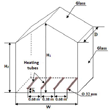
The considered physical problem is a model of an agricultural greenhouse submitted to different thermal conditions. We consider the case of closed greenhouse, taking into account convective and radiation exchanges which play an important role in greenhouse climate. The air in the greenhouse is considered as perfect gas (T = 300 K and P = 1 atm) and the medium is fully transparent. The dimensions of the model are represented in the Figure 1-a, with a height of H1 = 2 m, a width of W = 2.2 m and depth of D = 1.5 m.
The flow convection is caused by the buoyancy force in the greenhouse, the solar absorption on the ground and the heat flux from the contents of the heating tubes. The greenhouse heating is achieved by the circulation of a hot water in the tubes located near the ground at a height of h = 60 mm and a diameter Ǿ = 32 mm. The walls of the greenhouse are made by a semi-transparent material (glass) to reduce the absorption of thermal radiation with a thick of t = 4 mm.
As far as the boundary conditions concerned, we consider that the lateral, front and rear walls, as well as the ground have no heat exchange (adiabatic) that means that the heat flux is equal to zero. In the roof, we impose a constant temperature equal to T = 300 K. For the four tubes, we impose a constant heat flux equal to q = 100 W.m-2 for each tube. The heating of the greenhouse is done by the circulation of hot water in the tubes. In each case, we change the boundary conditions of the roof.
In the first case, we have imposed the temperature equal to T = 300 K. In the second case, we change the temperature by convective heat flux defined by:
$q=h\left(T-T_{0}\right)$ (1)
where, T0 = 300 K and the coefficient of heat transfer by convection is equal to h = 5 W.K-1.m-2. In the third case, we change only the heat transfer coefficient by h = 10 W.K-1.m-2. Then, in the fourth case, we have a mixed heat flux defined by convection and radiations, as follows:
$q=h\left(T-T_{0}\right)+\varepsilon \sigma\left(T^{4}-T_{0}^{4}\right)$ (2)
where, the heat transfer coefficient by convection is equal to h = 5 W.K-1.m-2, the ambient temperature is equal to T0 = 300 K, the external emissivity is equal to ε = 0.9 and the Stefan-Boltzmann constant is equal to σ = 5.672 10-8W.m-2.K-4. The equations systems describing governing the airflow under a greenhouse are the Navier-Stokes equations written in the dimensionless form as following:
$\frac{\partial u}{\partial x}+\frac{\partial v}{\partial y}+\frac{\partial w}{\partial z}=0$ (3)
$u \frac{\partial u}{\partial x}+v \frac{\partial u}{\partial y}+w \frac{\partial u}{\partial z}=-\frac{1}{\rho} \frac{\partial P}{\partial x}+\upsilon \left(\frac{\partial^{2} u}{\partial x^{2}}+\frac{\partial^{2} u}{\partial y^{2}}+\frac{\partial^{2} u}{\partial z^{2}}\right)$ (4)
$u \frac{\partial v}{\partial x}+v \frac{\partial v}{\partial y}+w \frac{\partial v}{\partial z}=-\frac{1}{\rho} \frac{\partial P}{\partial y}+\upsilon \left(\frac{\partial^{2} v}{\partial x^{2}}+\frac{\partial^{2} v}{\partial y^{2}}+\frac{\partial^{2} v}{\partial z^{2}}\right)+g \beta\left(T-T_{0}\right)$ (5)
$u \frac{\partial w}{\partial x}+v \frac{\partial w}{\partial y}+w \frac{\partial w}{\partial z}=-\frac{1}{\rho} \frac{\partial P}{\partial z}+\upsilon \left(\frac{\partial^{2} w}{\partial x^{2}}+\frac{\partial^{2} w}{\partial y^{2}}+\frac{\partial^{2} w}{\partial z^{2}}\right)$ (6)
Energy equation
$u \frac{\partial T}{\partial x}+v \frac{\partial T}{\partial y}+w \frac{\partial T}{\partial z}=\frac{k}{\rho C_{p}}\left(\frac{\partial^{2} w}{\partial x^{2}}+\frac{\partial^{2} w}{\partial y^{2}}+\frac{\partial^{2} w}{\partial z^{2}}\right)$ (7)
where, u, v, w, P, ρ, β, υ, k, Cp and T are respectively; the velocity component in Cartesians coordinates (x, y, z), pressure, density, thermal coefficient of expansion, kinematic viscosity, thermal conductivity, specific heat temperature.
To solve the problem, we have used the commercial CFD code Fluent. This code treats the general equations of the fluid dynamic as well as the energy conservation equation [16]. Also, it can describe the irradiative transfer operations within our arithmetic domain. It allows studying irregular field by considering the adequate mesh, boundary conditions and fluid characteristics. Figure 1-b shows the used mesh for the simulation. The distribution of points and meshes is symmetrically presented on the control volume. To do a test about the mesh density effect, we choose five meshes in the greenhouse with different sizes defined by 27000, 64000, 125000, 216000 and 343000 nodes. From comparison of different flow and heat parameters (Figure 1-c), we obtained a converged solution for the three girds size 125000, 216000 and 343000. For the further results, we are interested by the smaller mesh 125000 because it takes less time to calculate the solution.
a) Geometry
b) Meshing
(c) Mesh sensitivity test of the considered problem
Figure 1. Geometry, meshing, and mesh sensitivity test of the considered problem
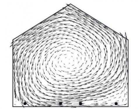
Figure 2 illustrates the comparison of the velocity vector field in the cavity obtained by our numerical computation and the experimental data of Roy et al. [5]. According to these results, the numerical results significantly reach a good agreement with the experimental data, since we find that the results are approximate the same.
In these conditions, a recirculation zone has been observed in the whole volume of the control volume.
a. Present results
b. Experimental data [5]
Figure 2. Velocity vector field: comparison of our results with those experimental data [5]
In this section, we present the numerical results of heat and fluid flow field in the greenhouse model subjected to different boundary thermal conditions, such as imposed temperature on the roof, flow convection, and mixed flow convection-radiation.
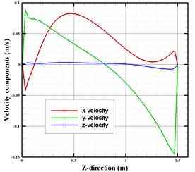
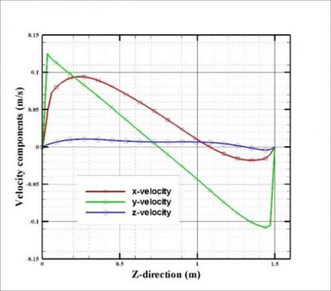
Figure 3, presents the profiles of the velocity components along the Z-axis at the middle plane of the greenhouse for the cases of the convective flux imposed on the roof (h = 5 W.K-1.m-2 and h = 10 W.K-1.m-2). From these results, it has been noted that the two cases have almost the same changes of velocity. However, it has been observed that the velocity in the case of the imposed convective flow with h = 10 W.K-1.m-2 is important than the case with h = 5 W.K-1.m-2. This means that when the heat transfer coefficient increases the velocity decreases.
Figure 4-a, illustrates the profile of X-velocity component along the Y-axis for the studied cases: h = 5 W.K-1.m-2, h = 10 W.K-1.m-2, mixed and T = 300 K of the heated greenhouse by the tubes. From these results, these profiles present the same space.
a. h = 5 W.K-1.m-²
b. h = 10 W.K-1.m-²
Figure 3. Profiles of the velocity components along the Z-axis at the middle plane of the greenhouse
The results show that the velocity values are high at the beginning of the greenhouse and decrease until reaching the value zero near the walls of the greenhouse end. The maximum value of the X-velocity component is obtained with the convective flow with h = 5 W.K-1.m-2 and h = 10 W.K-1.m-2 However, the minimum value is recorded in the case of the imposed temperature T = 300 K. In the imposed temperature case defined by T = 300 K, the velocity presents an intermediate value between the previous cases.
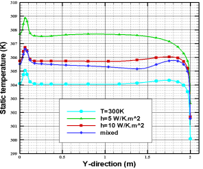
Figure 4-b, shows the profiles of the static temperature along the Y-axis for the considered cases in the greenhouse heated by the tubes. From these results, it has been observed that the profiles have the same pace, and show that the temperature values are high in the beginning of the greenhouse and decrease until reaching the value T = 300 K near the walls of the greenhouse end. The high value of the temperature is obtained in the case of a convective flow with h = 5 W.K-1.m-2. However, the low temperature is obtained in the case of an imposed temperature T = 300 K. The static temperature in the case of mixed flow and the case of convective flux with h = 10 W.K-1.m-2 are approximately the same.
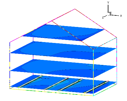
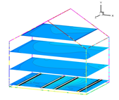
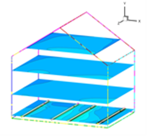
Figure 5, shows the isothermal surfaces in the planes defined by y = 0.06 m (level of tubes), y = 0.5 m, y =1 m and y = 1.5 m. In these conditions, the first plane y = 0.06 m corresponds to the level of tubes. Also, we have treated the cases defined by T = 300 K, h = 5 W.K-1.m-2, h = 10 W.K-1.m-2 and the mixed case. According to these results, it has been observed a small temperature variation in the greenhouse near the roof. However, a large temperature variation has been observed around the tubes, as they are the source of heat. For the first case, the average temperature in the greenhouse is between 303 K and 306 K. For the second case (h = 10 W.K-1.m-2), the average temperature in the greenhouse is between 305 K and 307 K. For the third case (h = 5 W.K-1.m-2), the average temperature is between 307 K and 309 K. However, for the last mixed case, the average temperature in the greenhouse is between 304 K and 307 K.
a. X-velocity component
b. Static temperature
Figure 4. Profiles of the X-velocity component along the Y-axis (a), and profiles of the static temperature along the Y-axis (b) at the middle plane of the greenhouse
(a) Case of imposed temperature on the roof
(b) Case of convective flux at the roof, for h = 10 W.K-1.m-2
(c) Case of convective flux at the roof, for h = 5 W.K-1.m-2
(d) Case of mixed flux at the roof
Figure 5. Isothermal surfaces in the greenhouse, for different studied cases
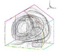
(a) Case of imposed temperature on the roof (Vavg = 13.05 cm/s)
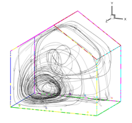
(b) Case of convective flux at the roof, for h = 5 W.K-1.m-2 (Vavg = 14.44 cm/s)
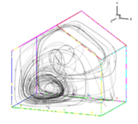
(c) Case of convective flux at the roof, for h = 10 W.K-1.m-2 (Vavg = 16.12 cm/s)
Figure 6. Some path lines in the greenhouse for different studied cases
Figure 6 shows the path lines of some fluid particles in the greenhouse, for the different boundary conditions defined bellow. According to these results, it has been observed that the particles circulate in counter clockwise direction forming several vortexes flow structures in all cases. For h = 5 W.K-1.m-2, the particles circulate in counter-clockwise direction forming one vortex flow structure in the bottom corner. For h = 10 W.K-1.m-2 and the last case, the particles circulate in counter clockwise direction forming one vortex flow structure in the middle of the greenhouse. In additions, the average velocity in the greenhouse is equal to Vavg = 13.05 cm/s in the first case and Vavg = 16.12 cm/s in the case of convective flux of h = 10 W.K-1.m-2. However, for h = 5 W.K-1.m-2, the average velocity in the greenhouse is equal to Vavg = 14.44 cm/s, and to Vavg = 13.48 cm/s in the case of the mixed flux.
In this paper, we have numerically studied the natural convection in a greenhouse by controlling the temperature and velocity of the air inside a closed greenhouse. Particularly, we have considered several configurations of thermal conditions to a greenhouse, like convection flux, imposed temperature and mixed flux. The main obtained results are given as follow:
These results help the farmers to set up a greenhouse with materials and dimensions suitable for external conditions.
The authors gratefully acknowledge the Directorate General of Scientific Research and Technological Development (DGSRTD)-to support this work, and fund the LME laboratory for carrying out research.
|
CP |
specific heat, J. kg-1. K-1 |
|
D |
depth of the green house enclosure, m |
|
g |
gravitational acceleration, m. s-2 |
|
H |
height of the greenhouse enclosure, m |
|
h |
coefficient of heat convection, W.m-2. K-1 |
|
k |
thermal conductivity, W.m-1. K-1 |
|
q |
convective heat flux, W |
|
T |
temperature, K |
|
u,v,w |
velocity components, m.s-1 |
|
x,y,z |
cartesian coordinates, m |
|
W |
width of the greenhouse enclosure, m |
|
Greek symbols |
|
|
β |
thermal expansion coefficient, K-1 |
|
ρ |
density, kg.m-3 |
|
υ |
kinematic viscosity, m-2. s-2 |
|
ε |
external emissivity |
|
σ |
Stefan-Boltzmann constant, W.m-2. K-4 |
|
Subscripts |
|
|
avg |
Average value |
[1] Boulard, T., Haxaire, R., Lamrani, M.A., Roy, J.C., Jaffrin, A. (1999). Characterization and modelling of the air fluxes induced by natural ventilation in a greenhouse. Journal of Agricultural Engineering Research, 74(2): 135-144. http://dx.doi.org/10.1006/jaer.1999.0442
[2] Boulard, T., Wang, S., Haxaire, R. (2000). Mean and turbulent air flows and microclimatic patterns in an empty greenhouse tunnel. Agricultural and Forest Meteorology, 100(2-3): 169-181. http://dx.doi.org/10.1016/S0168-1923(99)00136-7
[3] Bartzanas, T., Boulard, T., Kittas, C. (2002). Numerical simulation of the airflow and temperature distribution in a tunnel greenhouse equipped with insect-proof screen in the openings. Computers and Electronics in Agriculture, 34(1-3): 207-221. http://dx.doi.org/10.1016/S0168-1699(01)00188-0
[4] Chen, C.L., Cheng, C.H. (2002). Buoyancy-induced flow and convective heat transfer in an inclined arc-shape enclosure. International Journal of Heat and Fluid Flow, 23(6): 823-830. http://dx.doi.org/10.1016/S0142-727X(02)00189-3
[5] Roy, J.C., Bailly, Y., Boulard, T., Haxaire, R. (2000). Experimental study on natural convection in a heated greenhouse. Congrès de la Société Francaise des Thermique. Lyon, France. May 15–17, (Elsevier, Paris–Amsterdam), 11-17.
[6] Lebaal, C. (2008). Etude de la convection sous serres fermées et ouvertes en présence de la plante, Master’s Thesis, University of Batna, Algeria.
[7] Impron, I., Hemming, S., Bot, G.P.A. (2007). Simple greenhouse climate model as a design tool for greenhouses in tropical lowland. Biosystems Engineering, 98(1): 79-89. http://dx.doi.org/10.1016/j.biosystemseng.2007.03.028
[8] Tong, G., Christophe, D.M., Li, B. (2009). Numerical modelling of temperature variations in a Chinese solar greenhouse. Computers and Electronics in Agriculture, 68(1): 129-39. http://dx.doi.org/10.1016/j.compag.2009.05.004
[9] Fitz-Rodríguez, E., Kubota, C., Giacomelli, G.A., Tignor, M.E., Wilson, S.B., McMahon, M. (2010). Dynamic modeling and simulation of greenhouse environments under several scenarios: A web-based application. Computers and Electronics in Agriculture, 70(1): 105-116. http://dx.doi.org/10.1016/j.compag.2009.09.010
[10] Vadiee, A., Martin, V. (2012). Energy management in horticultural applications through the closed greenhouse concept, state of the art. Renewable and Sustainable Energy Reviews, 16(7): 5087-5100. http://dx.doi.org/10.1016/j.rser.2012.04.022
[11] Attar, I., Farhat, A. (2015). Efficiency evaluation of a solar water heating system applied to the greenhouse climate. Solar Energy, 119: 212-224. http://dx.doi.org/10.1016/j.solener.2015.06.040
[12] Hassanien, R.H.E., Li, M., Lin, W.D. (2016). Advanced applications of solar energy in agricultural greenhouses. Renewable and Sustainable Energy Reviews, 54: 989-1001. http://dx.doi.org/10.1016/j.rser.2015.10.095
[13] Taki, M., Ajabshirchi, Y., Ranjbar, S.F., Rohani, A., Matloobi, M. (2016). Modeling and experimental validation of heat transfer and energy consumption in an innovative greenhouse structure. Information Processing in Agriculture, 3(3): 157-174. http://dx.doi.org/10.1016/j.inpa.2016.06.002
[14] Taki, M., Rohani, A., Rahmati-Joneidabad, M. (2018). Solar thermal simulation and applications in greenhouse. Information Processing in Agriculture, 5(1): 83-113. http://dx.doi.org/10.1016/j.inpa.2017.10.003
[15] Zeroual, S., Bougoul, S., Benmoussa, H. (2018). Effect of radiative heat transfer and boundary conditions on the airflow and temperature distribution inside a heated tunnel greenhouse. Journal of Applied Mechanics and Technical Physics, 59(6): 1008-1014. http://dx.doi.org/10.1134/S0021894418060068
[16] Bouabdallah, S., Chati, D., Ghernaout, B., Atia, A., Laouirate, A. (2016). Turbulent mixed convection in enclosure containing a circular/square heat source. International Journal of Heat and Technology, 34(3): 446-454. http://dx.doi.org/10.18280/ijht.340314