Ancai Ma | Ping Tan* | Sheliang Wang | Fulin Zhou
© 2020 IIETA. This article is published by IIETA and is licensed under the CC BY 4.0 license (http://creativecommons.org/licenses/by/4.0/).
OPEN ACCESS
Under the action of earthquake, the dynamic interaction between the bridge pier and the surrounding water has a great impact on the dynamic response of the bridge structure. With a continuous sea-crossing beam bridge as an example, this paper studied the stochastic optimization of the parameters of nonlinear viscous damper and its damping performance under the fluid-solid coupling effect of waves and piers. In this study, a 2-degree-of-freedom bridge analysis model considering the fluid-solid coupling effect was constructed, and a nonlinear viscous damper was set in the model and subject to equivalent linearization according to the equivalent energy consumption criterion. Then on this basis, with minimizing the variance of the displacement of pier top as the target, this study applied the Lyapunov method to optimize the parameters of the damper, and explored its impact on the seismic response of the bridge and the damping performance considering the fluid-solid coupling effect. The research results showed that the fluid-solid coupling effect changed the dynamic characteristics of the bridge and increased its seismic response, and the viscous damper can effectively reduce the seismic response of the sea-crossing bridge and improve its damping performance.
continuous beam bridge, fluid-solid coupling effect, Morison equation, nonlinear viscous damper, stochastic optimization, damping performance
In recent years, the construction of sea-crossing bridges has shown an unprecedented growth trend. Sea-crossing bridges are often constructed in extremely complicated load environments. Under the action of earthquake, the fluid-solid coupling effect between the sea-crossing bridge piers and the surrounding water has a great impact on the dynamic response characteristics of the bridge structure [1-4], so the development of seismic reduction technology has very important engineering significance for improving the safety performance of sea-crossing bridges under the combined action of earthquakes and waves [5].
In the seismic response analysis of sea-crossing bridges, the fluid-soil coupling effect of waves and structures should be taken into account; under the action of loads such as earthquakes and waves, the fluid-solid coupling effect between bridge piers and waves would apply hydrodynamic pressure on the surface of bridge piers. In terms of hydrodynamic pressure calculation, researchers at home and abroad mainly use the simplified or the improved Morison equation [6-9]. Yamada et al. [10] adopted the modified Morison equation to calculate the hydrodynamic pressure and analyzed the dynamic response of the offshore pile structure under the action of earthquakes and waves. Based on the simplified Morison equation, Gao et al. [11] used the attached water mass to consider the influence of water. In terms of bridge damping, as a kind of damping device with high stability and good applicability, viscous dampers could be installed at appropriate positions on the bridge to reduce the seismic response of the bridge through damping energy consumption [12]. The optimization of damper parameters is a key link in the aseismic design. The traditional optimization method is mainly through the damping calculation of the structure under the action of deterministic ground motion, and then through the parameter sensitivity analysis to obtain the optimal damper parameters [13, 14]. However, in reality, earthquake is a random process, and deterministic analysis cannot accurately reflect its random characteristics, for this, Zhao et al. [15] used the frequency domain method of traditional random vibration analysis to simplified single-degree-of-freedom bridge system and optimized the parameters of viscous dampers for continuous beam bridges and suspension bridges. But the frequency domain method is only suitable for structures with lower degrees of freedom; so, in order to make it suitable for the stochastic optimization of structures with higher degrees of freedom, the nonlinear viscous dampers should be linearized first. Symans and Constantinou [16] proposed a damper linearization method based on equivalent energy consumption; Di Paola and Navarra [17] proposed a stochastic equivalent linearization method based on the minimum mean square error; since complex iterative operations are often involved in the solution process of stochastic equivalent linearization method, which is not conductive to application, therefore, this paper adopted the equivalent energy consumption linearization method to linearize the nonlinear viscous damper [18, 19].
This paper took a continuous sea-crossing beam bridge as the research object, and used the Morison equation to calculate the hydrodynamic pressure applied on the bridge pier by the fluid-solid coupling effect; a simplified analysis model of a 2-degree-of-freedom bridge considering the hydrodynamic pressure was proposed, a nonlinear viscous damper was set in the model, and the nonlinear viscous damper was equivalently linearized according to the equivalent energy consumption criterion; then on this basis, with minimizing the variance of the displacement of pier top as the target, the parameters of the damper was optimized by the Lyapunov equation method of the stochastic vibration analysis, and the impact of hydrodynamic pressure on reducing the seismic response of bridge and the shock absorption performance was studied.
This paper mainly consisted of the following contents: fluid-solid coupling effect of bridge piers, simplification of bridge analysis model, equivalent linearization of nonlinear viscous damper, motion equation for bridge damping, analysis of stochastic seismic response and derivation of extended state equation, optimization of damper parameters, and research of the shock absorption performance of bridges, etc.
The fluid-solid coupling effect between the bridge piers and the waves makes the structure surface subjected to the hydrodynamic pressure of the fluid under the action of earthquakes, waves and other dynamic forces. In the design of sea-crossing bridges, for small-diameter piers with a pier diameter / wave wavelength ratio < 0.2, the existence of the structure has no significant impact on the wave motion, and the Morison equation can be used to calculate the hydrodynamic pressure. This equation assumes that the sea water is an ideal, non-vortex, incompressible fluid, and that the presence of bridge piers in the water does not affect the wave motion, that is, the velocity and acceleration of the wave are still calculated by the adopted wave theory according to the original scale of the wave. The method believes that the force of water acting on the structure is mainly caused by the inertial force and resistance of the undisturbed acceleration field and velocity field acting on the structure along the direction of water movement. For cylindrical structures with relatively small lateral sizes, the hydrodynamic pressure on per unit length is:
$\begin{align} & F=\rho \frac{\pi {{D}^{2}}}{4}\ddot{u}+{{C}_{\text{m}}}\rho \frac{\pi {{D}^{2}}}{4}\left[ \ddot{u}-\left( {{{\ddot{x}}}_{\text{g}}}+\ddot{x} \right) \right] \\ & +\frac{1}{2}{{C}_{\text{d}}}\rho {{A}_{p}}\left[ \dot{u}-\left( {{{\dot{x}}}_{\text{g}}}+\dot{x} \right) \right]\left| \dot{u}-\left( {{{\dot{x}}}_{\text{g}}}+\dot{x} \right) \right| \\\end{align}$ (1)
where: ρ is the density of water; D is the length of the side of the cylinder facing the water; Ap is the projected area of the unit length of the cylinder perpendicular to the wave direction; $\dot{u}$ and $\ddot{u}$ are the velocity and acceleration of the wave; $\dot{x}$ and$\ddot{x}$ are the relative velocity and relative acceleration of the structure; ${{\dot{x}}_{\text{g}}}$ and ${{\ddot{x}}_{\text{g}}}$ are the velocity and acceleration of the ground; CM and CD are the inertial force coefficient and the drag force coefficient of the moving water.
Assuming the bridge is in still water, at this time $\dot{u}$=$\ddot{u}$=0, Formula (1) can be rewritten as:
$F=-{{C}_{M}}\rho \frac{\pi {{D}^{2}}}{4}({{\ddot{x}}_{\text{g}}}+\ddot{x})-\frac{1}{2}{{C}_{D}}\rho {{A}_{p}}({{\dot{x}}_{\text{g}}}+\dot{x})\left| {{{\dot{x}}}_{\text{g}}}+\dot{x} \right|$ (2)
The nonlinear resistance term in Formula (2) can be equivalently linearized by the least square method, and the obtained linearized Morison equation is:
$P=-\rho \left( {{C}_{M}}-1 \right)\frac{\pi }{4}{{D}^{2}}({{\ddot{x}}_{g}}+\ddot{x})-\frac{\rho }{2}{{C}_{D}}{{A}_{p}}\sqrt{\frac{8}{\pi }}({{\ddot{x}}_{g}}+\ddot{x}){{\sigma }_{{{{\ddot{x}}}_{g}}+\ddot{x}}}$ (3)
The motion equation of the bridge structure under the action of earthquake can be expressed as:
$\begin{align} & M\ddot{x}+C\dot{x}+Kx=-ME{{{\ddot{x}}}_{\text{g}}}-{{C}_{M}}\rho \frac{\pi {{D}^{2}}}{4}({{{\ddot{x}}}_{\text{g}}}+\ddot{x}) \\ & -\frac{1}{2}{{C}_{D}}\rho {{A}_{p}}({{{\dot{x}}}_{\text{g}}}+\dot{x})\left| {{{\dot{x}}}_{\text{g}}}+\dot{x} \right| \\\end{align}$ (4)
Compared with the inertial force, the resistance of the moving water is negligible, so Formula (4) can be further simplified and written as:
$M\ddot{x}+C\dot{x}+Kx=-ME{{\ddot{x}}_{\text{g}}}-{{M}_{w}}E({{\ddot{x}}_{\text{g}}}+\ddot{x})$ (5)
where, ${{M}_{w}}\text{=(}{{C}_{M}}-\text{1)}\rho \frac{\pi {{D}^{2}}}{4}$ is the attached moving water mass of the structure in the water.
By transposing the terms and sorting Formula (5) we can get:
$(M\text{+}{{M}_{w}})\ddot{x}+C\dot{x}+Kx=-(M+{{M}_{w}})E{{\ddot{x}}_{\text{g}}}$ (6)
where, M, C, K are the matrix of the structural mass, damping and stiffness, respectively; E is the index vector of the inertial force.
It can be seen from Formula (6) that when considering the effect of hydrodynamic pressure, it can be regarded as the attached moving water mass that moves with the structure. In the formula, the inertial force coefficient of the moving water is related to the shape of the structure, for the cylindrical piers, it could take CM=2.
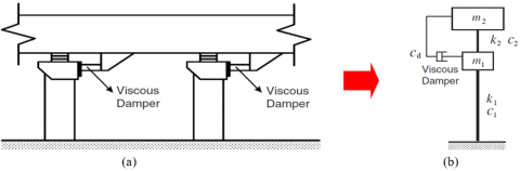
For a regular continuous beam bridge, it can be simplified to a 2-degrees-of-freedom model shown in Figure 1, the model can be used to reflect its dynamic response characteristics well under the action of earthquakes [20].
Figure 1. A simplified bridge model with viscous dampers
First, the bridge pier was simplified to a single mass-point system; then together with the rigidity and damping of the support, and the mass of the beam, they constituted a two mass-point system. For the pier which is in a complete elastic state, when both shear deformation and bending deformation are taken into consideration, the combined stiffness is:
${{k}_{1}}\text{=}\frac{\text{1}}{\frac{1}{{{k}_{b}}}+\frac{1}{{{k}_{v}}}}\text{=}\frac{1}{\frac{{{H}^{\text{3}}}}{3E{{I}_{z}}}+\frac{H}{{{A}_{v}}G}}$ (7)
where, kb is the bending stiffness, kv is the shear stiffness, H is the height of the pier, Iz is the inertia moment of the pier section, Av is the shear area of the pier, E is the elastic modulus, G is the shear modulus.
When the distributed mass of the pier is equivalent to the mass of the pier top, assuming that the deformation of the pier conforms to a parabola, then its deformation function is:
$\psi (z)\text{=(}\frac{3{{z}^{2}}}{2{{H}^{2}}}-\frac{{{z}^{3}}}{2{{H}^{3}}})$ (8)
When distributed mass of the pier is known to be ${{\bar{m}}_{c}}(z)$, the distributed mass concentrating on the top of the pier forms an additional mass on the pier:
$\begin{align} & {{m}^{*}}=\int_{0}^{H}{{{{\bar{m}}}_{c}}(z)}{{\psi }^{2}}(z)dz \\ & =\int_{0}^{H}{{{{\bar{m}}}_{c}}(z)}{{(\frac{3{{z}^{2}}}{2{{H}^{2}}}-\frac{{{z}^{3}}}{2{{H}^{3}}})}^{2}}dz \\ & =\frac{3}{8}{{{\bar{m}}}_{c}}H \\\end{align}$ (9)
The hydrodynamic pressure acts on the bridge pier as distributed load. First, the distributed hydrodynamic pressure on unit pier was converted into the equivalent node load on the pier top; then, to facilitate the use of the simplified Morison equation, the equivalent node load on the pier top was converted into the mass of the additional moving water on the pier top [21].
The damping force of the nonlinear viscous damper can be expressed as:
$F_{D}=c_{\alpha}|\dot{v}|^{\alpha} \operatorname{sgn}(\dot{v})$ (10)
where, FD is the damping force; cα is the damping coefficient; α is the velocity index, its value range is 0.3~0.5; $\dot{v}$ is the relative velocity at both ends of the damper; $\operatorname{sgn}(\cdot)$ is a sign function.
The linearization criterion is that the energy consumed in one cycle of nonlinear viscous damping is equal to the energy consumed in one cycle of the equivalent damping, then the equivalent damping coefficient of the viscous damper could be obtained as:
${{c}_{e}}=\lambda {{c}_{\alpha }}{{\omega }^{\alpha -1}}v_{0}^{\alpha -1}/\pi $ (11)
where, ce is the equivalent damping coefficient; ω is the circular frequency corresponding to the harmonic excitation; v0 is the maximum displacement loaded by the damper; then the expression of λ is:
$\lambda ={{2}^{\text{2+}\alpha }}{{\Gamma }^{2}}\left( 1+\alpha /2 \right)/\Gamma \left( 2+\alpha \right)$ (12)
where, Γ(⋅) is a gamma function.
After viscous damper is installed, the motion equation of the bridge under the action of earthquake is:
$\begin{align} & (M+{{M}_{w}})\ddot{x}(t)+(C\text{+}{{C}_{\text{e}}})\dot{x}(t)+Kx(t) \\ & =-(M+{{M}_{w}})E{{{\ddot{x}}}_{g}}(t) \\\end{align}$ (13)
where, Ce is the additional damping matrix when viscous dampers have been installed.
Then motion equation (13) could be rewritten in the form of the structure’s state space:
${{\mathbf{\dot{Y}}}_{s}}={{\mathbf{A}}_{s}}{{\mathbf{Y}}_{s}}+{{\mathbf{B}}_{s}}{{\ddot{x}}_{g}}\left( t \right)$ (14)
where,
${{\mathbf{Y}}_{s}}=\left\{ \begin{matrix} x \\ {\dot{x}} \\\end{matrix} \right\}$,
${{\mathbf{A}}_{s}}=\left[ \begin{matrix} \mathbf{0} & \mathbf{I} \\ -{{(M+{{M}_{w}})}^{-1}}\mathbf{K} & -{{(M+{{M}_{w}})}^{-1}}(C\text{+}{{C}_{\text{e}}}) \\\end{matrix} \right]$,
${{\mathbf{B}}_{s}}=\left\{ \begin{matrix} \mathbf{0} \\ -{{(M+{{M}_{w}})}^{-1}}E \\\end{matrix} \right\}$
For the 2-degree of freedom model:
$M=\left[ \begin{matrix} {{m}_{1}} & \text{0} \\ \text{0} & {{m}_{\text{2}}} \\\end{matrix} \right]$, ${{M}_{w}}=\left[ \begin{matrix} {{m}_{w}} & \text{0} \\ \text{0} & 0 \\\end{matrix} \right]$,
$C\text{=}\left[ \begin{matrix} {{c}_{1}}+{{c}_{2}} & -{{c}_{2}} \\ -{{c}_{2}} & {{c}_{2}} \\\end{matrix} \right]$,
${{C}_{e}}\text{=}\left[ \begin{matrix} {{c}_{e}} & -{{c}_{e}} \\ -{{c}_{e}} & {{c}_{e}} \\\end{matrix} \right]$,
$K=\left[ \begin{matrix} {{k}_{1}}+{{k}_{2}} & -{{k}_{2}} \\ -{{k}_{2}} & {{k}_{2}} \\\end{matrix} \right]$ (15)
where, m1=m* is the additional mass on the pier top, m2 is the concentrated mass of the upper structure of the bridge beam, mw is the converted mass of additional moving water on the pier top; c1 and c2 are respectively the damping coefficient of the pier and the damping coefficient of the support; k1 and k2 are respectively the equivalent stiffness of the pier and the equivalent stiffness of the support.
In this paper, the Clough-Penzien model was taken as the seismic excitation spectrum for the analysis of the structure’s stochastic seismic response. The model treated the ground soil layer as two single-degree-of-freedom linear filters. According to Lin et al. [22], the filter equation of the Clough-Penzien model can be expressed as:
$\begin{align} & {{{\ddot{u}}}_{g}}\left( t \right)+2{{\xi }_{g}}{{\omega }_{g}}{{{\dot{u}}}_{g}}\left( t \right)+\omega _{g}^{2}{{u}_{g}}\left( t \right)=-w\left( t \right) \\ & {{{\ddot{x}}}_{g}}\left( t \right)+2{{\xi }_{f}}{{\omega }_{f}}{{{\dot{x}}}_{g}}\left( t \right)+\omega _{f}^{2}{{x}_{g}}\left( t \right)=-{{{\ddot{x}}}_{f}}\left( t \right) \\ & {{{\ddot{x}}}_{f}}\left( t \right)={{{\ddot{u}}}_{g}}\left( t \right)+w\left( t \right) \\\end{align}$ (16)
where, ωg and ξg are parameters of the first filter of the ground soil layer, ug(t) is the response of the first filter, ${{\ddot{x}}_{f}}\left( t \right)$ is the corresponding absolute acceleration; ωf and ξf are parameters of the second filter of the ground soil layer, w(t) is the white noise excitation of the bedrock, ${{\ddot{x}}_{g}}\left( t \right)$ is the ground acceleration of the spectral model.
Above formulas can be combined and written as the state space equation of the excitation:
${{\mathbf{\dot{Y}}}_{g}}={{\mathbf{A}}_{g}}{{\mathbf{Y}}_{g}}+{{\mathbf{B}}_{g}}w\left( t \right)$ (17)
where,
${{\mathbf{A}}_{g}}=\left[ \begin{matrix} \mathbf{0} & \mathbf{I} \\ -\mathbf{M}_{g}^{-1}{{\mathbf{K}}_{g}} & -\mathbf{M}_{g}^{-1}{{\mathbf{C}}_{g}} \\\end{matrix} \right]$, ${{\mathbf{B}}_{g}}=\left\{ \begin{matrix} \mathbf{0} \\ -\mathbf{M}_{g}^{-1}{{\mathbf{I}}_{g}} \\\end{matrix} \right\}$,
${{\mathbf{Y}}_{g}}=\left\{ \begin{matrix} {{\mathbf{z}}_{g}} \\ {{{\mathbf{\dot{z}}}}_{g}} \\\end{matrix} \right\}$, ${{\mathbf{M}}_{g}}=\left[ \begin{matrix} 1 & 1 \\ 0 & 1 \\\end{matrix} \right]$,
${{\mathbf{C}}_{g}}=\left[ \begin{matrix} 2{{\xi }_{f}}{{\omega }_{f}} & 0 \\ 0 & 2{{\xi }_{g}}{{\omega }_{g}} \\\end{matrix} \right]$, ${{\mathbf{K}}_{g}}=\left[ \begin{matrix} \omega _{f}^{2} & 0 \\ 0 & \omega _{g}^{2} \\\end{matrix} \right]$,
${{\mathbf{I}}_{g}}=\left\{ \begin{matrix} 1 \\ 1 \\\end{matrix} \right\}$, ${{\mathbf{z}}_{g}}=\left\{ \begin{matrix} {{x}_{g}} \\ {{u}_{g}} \\\end{matrix} \right\}$
The state equation of the excitation (17) and the state equation of the structure (14) could be combined and written as an extended state space equation:
$\mathbf{\dot{Y}}=\mathbf{AY}+\mathbf{B}w\left( t \right)$ (18)
where,
$\mathbf{A}=\left[ \begin{matrix} {{\mathbf{A}}_{s}} & {{\mathbf{B}}_{s}}{{\mathbf{T}}_{g}}{{\mathbf{A}}_{g}} \\ \mathbf{0} & {{\mathbf{A}}_{g}} \\\end{matrix} \right]$, $\mathbf{B}=\left[ \begin{matrix} {{\mathbf{B}}_{s}}{{\mathbf{T}}_{g}}{{\mathbf{B}}_{g}} \\ {{\mathbf{B}}_{g}} \\\end{matrix} \right]$,
$\mathbf{Y}=\left\{ \begin{matrix} {{\mathbf{Y}}_{s}} \\ {{\mathbf{Y}}_{g}} \\\end{matrix} \right\}$, ${{\mathbf{T}}_{g}}=[0,0,1,0]$
Order the variance matrix of the response to be ${{\mathbf{E}}_{Y}}=E\left( \mathbf{Y}{{\mathbf{Y}}^{T}} \right)$, and ${{\mathbf{E}}_{g}}=\mathbf{B}2\pi {{S}_{0}}{{\mathbf{B}}^{T}}$ is the covariance matrix of the input excitation, wherein S0 is the spectral density of the bedrock excitation$w$, then the Lyapunov equation describing the response variance can be obtained as:
$\frac{d{{\mathbf{E}}_{Y}}}{dt}=\mathbf{A}{{\mathbf{E}}_{Y}}+{{\mathbf{E}}_{Y}}{{\mathbf{A}}^{T}}+{{\mathbf{E}}_{g}}$ (19)
When the excitation is steady state, the response variance is independent of time, and the above formula becomes:
$\mathbf{A}{{\mathbf{E}}_{Y}}+{{\mathbf{E}}_{Y}}{{\mathbf{A}}^{T}}+{{\mathbf{E}}_{g}}=0$ (20)
The response variance of the structure could be obtained by solving the above formula.
From the calculation formula of damping force (10) we can know that when the velocity index α and damping coefficient cα of the viscous damper take different values, the influence on the response of the structure is also different. Therefore, in the damping design, the parameters α and cα of the viscous damper installed on the bridge should be optimized; and studying the influence of the change of parameters on the response of the structure could provide references for the determination of the parameters of the damper.
From the perspective of improving the safety performance of the structure, minimizing the squared variance of the displacement of pier top was taken as the optimization goal, that is:
$\begin{align} & \underset{{{c}_{\alpha }},\alpha }{\mathop{\min }}\,\sigma _{{{x}_{p}}}^{\text{2}}({{c}_{\alpha }},\alpha ) \\ & s.t.:{{c}_{\alpha }}_{\min }\le {{c}_{\alpha }}\le {{c}_{\alpha }}_{\max } \\ & {{\alpha }_{\min }}\le \alpha \le {{\alpha }_{\max }} \\\end{align}$ (21)
where, cαmin and cαmax are the lower limit and upper limit of the damping coefficient, respectively; αmin and αmax are the lower limit and upper limit of the damping index, respectively.
Taking a continuous sea-crossing beam bridge as an example, two sets of viscous dampers were installed between the pier top and the beam body, and the proposed method was applied to the damping optimization of the viscous dampers. The bridge piers were cylindrical solid piers with a diameter of 3.0 m, the height of the piers was 28.2 m, the water depth was 20 m. The mass of two adjacent half-spans of the pier m2=500,000 kg was taken as the mass of the superstructure, which acted on the support in the form of concentrated mass, and the elastic modulus of the pier was 3.0×10⁴ MPa, the equivalent stiffness was 1.587×10⁷ N/m, the concentrated mass of the pier body equivalent to the pier top was 186880 kg, the equivalent stiffness of the support was 7.69×10⁶ N / m, the damping ratio of the structure took 0.05, and the damping ratio of the support took 0.10. The seismic precautionary intensity of the bridge was 8 degrees, the designed basic earthquake acceleration was 0.2g, the site category was category II, and the design earthquake group was the second group; In the stochastic response analysis, the Clough-Penzien spectral parameters were calculated by the method of [23] Marano et al. [23]. The one-sided spectral density of the bedrock was S0=13.336 cm2/(rad•s3), ωg=15.7 rad/s, ξg=0.72, it took ξf=ξg, ωf=0.15ωg rad/s.
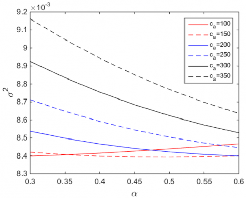
Figure 2. Change of pier top displacement variance with damping coefficient cα
Figure 3. Change of pier top displacement variance with velocity index α
Through the analysis of the stochastic seismic response, the relationship between the squared variance of the pier top displacement of the bridge and the damping coefficient cα, and the relationship between the squared variance of the pier top displacement of the bridge and the velocity index α are shown in Figures 2 and 3.
It can be seen from Figure 2 that, with the increase of the damping coefficient cα, the variance of the displacement of the pier top decreased first and then gradually increased; for curves of different α values, they generally approached the minimum values around cα=1.5×10⁵.
From Figure 3, it can be seen that, overall, the variance of the displacement of the pier top decreased with the increase of the velocity index α. Only the curve with cα=1.5×10⁵ reached the minimum value near the velocity index α=0.45. Through comprehensive comparison, α=0.45 and cα=1.5×10⁵ were selected as the optimal damper parameters of the bridge.
In order to analyze the damping effect of viscous dampers on the bridge under the coupling of earthquake and hydrodynamic pressure, the damping parameters obtained by the above optimization method were adopted, and the El Centro waves were used to analyze the structure's time-history response. The importance coefficient of the structure took 1.7. Table 1 lists the first-order and second-order frequencies under two conditions: considering the effect of hydrodynamic pressure (with water), and doesn’t considering the effect of hydrodynamic pressure (without water). It can be seen that, after the fluid-solid coupling effect had been taken into account, the first-order frequency was reduced by 0.6% and the second-order by 9.9%, indicating that the presence of water had changed the dynamic characteristics of the structure.
Table 1. Natural vibration frequency of the bridge
|
Order of the frequency |
Frequency without water (Hz) |
Frequency with water (Hz) |
Change rate (%) |
|
1 |
3.152 |
3.134 |
-0.6 |
|
2 |
11.470 |
10.334 |
-9.9 |
In order to analyze the effect of fluid-solid coupling on the seismic response of the bridge, for the seismic response of the structure without dampers, two situations of with water (considering the effect of hydrodynamic pressure) and without water (doesn’t considering the effect of hydrodynamic pressure) were calculated. Table 2 lists the horizontal displacement of the pier top, the displacement of the support, the bending moment of pier bottom, and the shear force of pier bottom under the two situations and their change rates. Figure 4 shows the time-history curves of the horizontal displacement of the pier top and the bending moment of the pier bottom. It can be seen from the figure that: after the fluid-solid coupling effect had been taken into account, the pier top displacement, the bending moment of pier bottom, and the shear force of pier bottom increased by about 10.8%, and the support displacement increased by 7.2%. Under the action of earthquake, the seismic response of bridge piers in the water was obviously affected by the fluid-solid coupling. The existence of hydrodynamic pressure amplified the dynamic response of the bridge. Therefore, for the sea-crossing bridges, it is necessary to consider the fluid-solid coupling effect in the seismic design.
Table 2. Seismic response peaks of the bridge with/without water
|
Without water |
With water |
Change rate (%) |
|
|
Pier top displacement (mm) |
60.0 |
66.5 |
10.8 |
|
Support deformation (mm) |
91.1 |
97.7 |
7.2 |
|
Bending moment of pier bottom (kN.m) |
27255 |
30170 |
10.7 |
|
Shear force of pier bottom (kN) |
953 |
1056 |
10.8 |
(a) Pier top displacement
(b) Bending moment of pier bottom
Figure 4. Time-history curves of seismic response of bridge with/without water
In order to measure the control effect, the concept of vibration reduction rate was introduced, which is defined as follows:
${{R}_{i}}\text{=}\frac{{{\left| d_{i}^{u}(t) \right|}_{\max }}-{{\left| d_{i}^{c}(t) \right|}_{\max }}}{{{\left| d_{i}^{u}(t) \right|}_{\max }}}\times 100%$ (22)
where, Ri is the vibration reduction rate of the i-th degree of freedom, $d_{i}^{u}(t)$ and $d_{i}^{c}(t)$ are respectively the seismic response of the i-th degree of freedom of the structure under earthquake resistance and shock absorption conditions.
Table 3 lists the displacement of the pier top, the displacement of the support, the bending moment of pier bottom, and the shear force of pier bottom of the bridge and their change rates considering the fluid-solid coupling effect under earthquake resistance and damping performance. Figure 5 gives the corresponding time-history curves. It can be seen from the figure that: for bridge with viscous dampers installed and fluid-solid coupling effect taken into account, the vibration reduction rates of pier top displacement, pier bottom bending moment and pier bottom shear force were between 12.3% and 14.3%, and the vibration reduction rate of support displacement was 26.7%. The viscous damper designed in this paper had obvious effects on the damping performance of bridge piers, and its damping performance effect on the support displacement was especially significant. Using viscous dampers in the seismic control of sea-crossing bridges can effectively reduce the seismic response of the structure and improve the seismic safety of the bridge.
Table 3. Comparison of seismic control effects considering hydrodynamic pressure
|
Without damper |
With damper |
Vibration reduction rate (%) |
|
|
Pier top displacement (mm) |
66.5 |
58.3 |
12.3 |
|
Support deformation (mm) |
97.7 |
71.6 |
26.7 |
|
Bending moment of pier bottom (kN.m) |
30170 |
26414 |
12.4 |
|
Shear force of pier bottom (kN) |
1056 |
905 |
14.3 |
(a) Pier top displacement
(b) Support deformation
(c) Bending moment of pier bottom
(d) Shear force of pier bottom
Figure 5. Time-history curves of seismic response of bridge considering the effect of hydrodynamic pressure
(1) With the increase of the damping coefficient, the variance of the displacement of the pier top decreased first and gradually increased later, and the velocity exponential curves generally approached the minimum values around cα=1.5×10⁵. Overall, the variance of the displacement of the pier top decreased with the increase of the velocity index α. Only the curve with cα=1.5×10⁵ reached the minimum value near the velocity index α=0.45. At last, α=0.45 and cα=1.5×10⁵ were selected as the optimal damper parameters of the bridge.
(2) After the fluid-solid coupling effect was taken into account, the first-order frequency of the bridge was reduced by 0.6% and the second-order by 9.9%. The presence of water had changed the dynamic characteristics of the bridge structure.
(3) After the fluid-solid coupling effect was taken into account, the pier top displacement, the bending moment of pier bottom, and the shear force of pier bottom generally increased by about 10.8%, and the support displacement increased by 7.2%. Under the action of earthquake, the seismic response of bridge piers in the water was obviously affected by the fluid-solid coupling. The existence of hydrodynamic pressure amplified the dynamic response of the bridge. Therefore, for the sea-crossing bridges, it is necessary to consider the fluid-solid coupling effect in the seismic design.
(4) For bridge with viscous dampers installed and fluid-solid coupling effect taken into account, the vibration reduction rates of pier top displacement, pier bottom bending moment and pier bottom shear force were between 12.3% and 14.3%, and support displacement was 26.7%. The installation of viscous dampers had obvious effects on the damping performance of bridge piers, especially on the support displacement. Using viscous dampers can effectively reduce the seismic response of sea-crossing bridges, and improve the seismic safety of the bridges.
This work is supported by the National Key Research and Development Project (Grant No.: 2017YFC0703600); Ministry of Education Innovation Team Project (Grant No.: IRT13057); National Natural Science Foundation of China (Grant No.: 51678480).
[1] Li, Z.X., Wu, K., Shi, Y., Ning, L., Yang, D. (2019). Experimental study on the interaction between water and cylindrical structure under earthquake action. Ocean Engineering, 188: 106330. https://doi.org/10.1016/j.oceaneng.2019.106330
[2] Zhang, S.W., Tao, X.X., Liu, H.M. (2018). Seismic hydrodynamic pressure of bridge pier in deep water. Advances in Engineering Research, 120: 1784-1787. https://doi.org/10.2991/ifeesm-17.2018.323
[3] Zhou, Y., Sun, L. (2019). Effects of environmental and operational actions on the modal frequency variations of a sea-crossing bridge: A periodicity perspective. Mechanical Systems and Signal Processing, 131: 505-523. https://doi.org/10.1016/j.ymssp.2019.05.063
[4] Qi, Y., Wang, F. (2019). Method for Structural Damage Identification of Reinforced Concrete of Sea-crossing Bridge. Journal of Coastal Research, 97(S1): 88-92. https://doi.org/10.2112/SI97-011.1
[5] Wu, A.J., and Yang, W.L. (2020). Numerical study of pile group effect on the hydrodynamic force on a pile of sea-crossing bridges during earthquakes. Ocean Engineering, 199: 106999. https://doi.org/10.1016/j.oceaneng.2020.106999
[6] Nasim, M., Setunge, S., Zhou, S., Mohseni, H. (2019). An investigation of water-flow pressure distribution on bridge piers under flood loading. Structure and Infrastructure Engineering, 15(2): 219-229. https://doi.org/10.1080/15732479.2018.1545792
[7] Mondal, S., Wu, C.H., Sharma, M.M. (2016). Coupled CFD-DEM simulation of hydrodynamic bridging at constrictions. International Journal of Multiphase Flow, 84: 245-263. https://doi.org/10.1016/j.ijmultiphaseflow.2016.05.001
[8] Yuan, Y., Wei, W., Igarashi, A., Tan, P., Iemura, H., Zhu, H. (2017). Experimental and analytical studies of seismic response of highway bridges isolated by rate-dependent rubber bearings. Engineering Structures, 150: 288-299. https://doi.org/10.1016/j.engstruct.2017.06.020
[9] Beji, S. (2019). Applications of Morison's equation to circular cylinders of varying cross-sections and truncated forms. Ocean Engineering, 187: 106156. https://doi.org/10.1016/j.oceaneng.2019.106156
[10] Yamada, Y., Iemura, H., Kawano, K., Venkataramana, K. (1989). Seismic response of offshore structures in random seas. Earthquake Engineering & Structural Dynamics, 18(7): 965-981. https://doi.org/10.1002/eqe.4290180704
[11] Gao, X.K., Zhu, X. (2006). Hydrodynamic effect on seismic response of bridge pier in deep water. Journal of Beijing Jiaotong University, 30(1): 55-58. https://doi.org/10.3969/j.issn.1673-0291.2006.01.014
[12] Guo, W., Li, J.Z., Guan, Z.G. (2019). Shake table studies of the longitudinal seismic mitigation effect of viscous dampers on a kilometer-scale cable-stayed bridge. China Journal of Highway and Transport, 32(11): 156-164. https://doi.org/10.19721/j.cnki.1001-7372.2019.11.015
[13] Mesbahi, J., Malek, A., Salimbahrami, B. (2016). Robust control synchronization on multi-story structure under earthquake loads and random forces using H∞ algorithm. Biquarterly Research Journal of Control and Optimization in Applied Mathematics, 1(2): 39-52.
[14] Heo, G., Kim, C., Jeon, S., Lee, C., Jeon, J. (2017). A hybrid seismic response control to improve performance of a two-span bridge. Structural Engineering and Mechanics, 61(5): 675-684. https://doi.org/10.12989/sem.2017.61.5.675
[15] Zhao, G.H., Liu, J.X., Li, Y. (2013). Parameter optimization of fluid viscous damper based on stochastic vibration. Journal of Southwest Jiaotong University, 48(6): 1002-1007. https://doi.org/10.3969/j.issn.0258-2724.2013.06.006
[16] Symans, M.D., Constantinou, M.C. (1997). Seismic testing of a building structure with a semi‐active fluid damper control system. Earthquake Engineering & Structural Dynamics, 26(7): 759-777. https://doi.org/10.1002/(SICI)1096-9845(199707)26:7<759::AID-EQE675>3.0.CO;2-E
[17] Di Paola, M., Navarra, G. (2009). Stochastic seismic analysis of MDOF structures with nonlinear viscous dampers. Structural Control and Health Monitoring, 16(3): 303-318. https://doi.org/10.1002/stc.254
[18] Alibrandi, U., Mosalam, K.M. (2017). Equivalent linearization methods for stochastic dynamic analysis using linear response surfaces. Journal of Engineering Mechanics, 143(8): 04017055. https://doi.org/10.1061/(ASCE)EM.1943-7889.0001264
[19] Anh, N.D., Linh, N.N. (2018). A weighted dual criterion of the equivalent linearization method for nonlinear systems subjected to random excitation. Acta Mechanica, 229(3): 1297-1310. https://doi.org/10.1007/s00707-017-2009-y
[20] Erkus, B., Abé, M., Fujino, Y. (2002). Investigation of semi-active control for seismic protection of elevated highway bridges. Engineering Structures, 24(3): 281-293. https://doi.org/10.1016/S0141-0296(01)00095-5
[21] Ding, Y., Ma, R., Shi, Y.D., Li, Z.X. (2018). Underwater shaking table tests on bridge pier under combined earthquake and wave-current action. Marine Structures, 58: 301-320. https://doi.org/10.1016/j.marstruc.2017.12.004
[22] Lin, B.C., Tadjbakhsh, I.G., Papageorgiou, A.S., Ahmadi, G. (1989). Response of base-isolated buildings to random excitations described by the Clough-Penzien spectral model. Earthquake engineering & structural dynamics, 18(1): 49-62. https://doi.org/10.1002/eqe.4290180106
[23] Marano, G.C., Trentadue, F., Morrone, E., Amara, L. (2008). Sensitivity analysis of optimum stochastic nonstationary response spectra under uncertain soil parameters. Soil Dynamics and Earthquake Engineering, 28(12): 1078-1093. https://doi.org/10.1016/j.soildyn.2007.12.003