Hanane Maria Regue* | Belkacem Bouali | Toufik Benchatti | Ahmed Benchatti
© 2020 IIETA. This article is published by IIETA and is licensed under the CC BY 4.0 license (http://creativecommons.org/licenses/by/4.0/).
OPEN ACCESS
This paper presents a numerical simulation of the conjugate heat transfer and fluid flow in the tube absorber of a parabolic trough collector (PTC). The main objective is to analyze the system performance with and without a secondary reflector. The PTC is tested under climatic conditions present in Laghouat city (ALGERIA). PVSYST software is used to provide numerical temporal values of the solar heat flux in Laghouat region. Daily heat flux values for four days in different seasons have been taken. The non-uniform heat flux distribution on the absorber tube is calculated by using Monte Carlo ray tracing method in SolTrace software. The governing equations of fluid flow and heat transfer in the system are solved by using ANSYS-CFX CFD software. A comparison between two cases (with and without second reflector) with the same working fluid (Therminol VP-1) is carried out. The obtained results show that the maximum fluid temperatures are reached during the month of June while the minimum values are obtained on the month of December. However, the system performance is practically the same for the four seasons. Moreover, the performance of the system with a secondary collector is better than that without a secondary reflector with a ratio of about 3/2.
solar thermal energy, solar parabolic trough collector, secondary reflectors, receiver tube, conjugate heat transfer simulation
Sustainable renewable energy comes from sources such as hydro, sunlight or wind. Natural replenishment of these resources allows them to be classified as “renewable”, inexhaustible, and can never be depleted [1]. Improving system efficiencies as well as reduction in the cost of manufacture have contributed to an increased focus on the development of concentrating solar power systems (CPC) [2]. Thus, many researchers have been working in this field trying new ideas and optimizing the existing collectors [3], particularly in their application in steam generation for solar thermal power plants. One of the main solar energy collectors is the Parabolic Trough Collector (PTC). A PTC includes an evacuated tube and a linear parabolic reflector. The evacuated tube is located on the focal line of the parabolic reflector (reflective material bent into a parabolic shape). Thereby, the concentrated solar beam heats the working fluid within the tube. The ability to generate energy over a wide temperature with limited deterioration in efficiency further emphasizes the PTC importance in solar energy generation [4]. The performance of a solar thermal energy conversion system is affected by the collector, the absorber and the concentrator. The operation of these components is governed by the following parameters: optical properties, heat transfer fluid (HTF) properties, inlet temperature, flow rate of HTF, solar insolation, wind speed, and atmospheric temperature. Outputs include collector efficiency, HTF outlet temperature, heat gain, and heat/optical losses [5].
Many academic studies have been conducted on the numerous types of solar thermal collector and their applications. Details on the wide variety of uses for solar energy collectors, costs, and environmental benefits are presented by Kaligirou [6]. Zou et al. [7] studied the theoretical optical performance of the parabolic trough solar collector. Xiao et al. [8] simulated the heat flux distribution on the outer surface of the absorber tube of a parabolic solar collector receiver based on the Monte-Carlo Ray Trace method. The Monte Carlo Method was also used by Larger Liang et al. [9] to analyze the solar flux distribution on the receiver and the optical thermal performance of the parabolic trough collector. Eck and Hirsch [10] performed a transient simulation of direct steam generation collector loops in combination with a control system.
On the other hand, many experimental studies have been conducted with emphasis on various aspects of the PTC. Examples include Gang et al. [11] who conducted an experimental investigation on exergy efficiency and overall thermal efficiency of the compound parabolic collector; and Ceylan and Ergun [12] who carried out an experimental study of a temperature-controlled CPC, and reported energy efficiency and exergy efficiency.
Some researchers have also concentrated their efforts on adding another reflector. Several attempts of second stage reflectors for PTCs [13-17] have included complicated secondary mirror geometries that, while increasing the concentration ratio considerably, did not become practical solutions due to the difficulty for manufacturers in building them at a competitive cost. Recent work states the potential improvement of secondary reflectors in PTC and analyses geometries previously investigated [18]. A new method for the design of the secondary mirror has been carried out by Canavarro et al. [19]. Another study using secondary reflector in linear absorbers are described in reference [15].
In this paper, a numerical simulation of the conjugate heat transfer and fluid flow in the absorber tube of a PTC prototype [20] is performed. The PTC is tested under climatic conditions present in Laghouat city (ALGERIA). PVSYST software is used to provide numerical temporal values of the solar heat. A secondary reflector is studied as a solution to increase the geometrical concentration ratio. As an additional advantage, the secondary reflector helps to distribute the energy flux around the tube more evenly than with a classic PTC (without secondray reflector). This uniforme distribution [20] could help to minimize the reflection and radiation losses and could also stabilize internal two phase flow and pressure drop. In order to do comparison between classic PTC and PTC with secondary reflector, the PTC receiver analysis has been carried out by using non-uniform and uniforme heat flux distributions on the surface of the absorber tube. Monte Carlo ray tracing method in SolTrace software is used to calculate the flux distribution in each case. The governing equations of fluid flow and heat transfer in the system are solved by using ANSYS-CFX CFD software.
A PTC is a line-focusing system that uses a parabolic reflector to concentrate solar radiation onto a linear receiver. Reflector is one of the vital parts of the PTC as it decides the fraction of solar irradiance to be collected by the absorber tube. The system considered in this work is a prototype described in our previous paper [20]. The PTC has a length of 2 m and an area of 2×2 m2.


Figure 1. PTC module with secondary reflector
We have introduced a secondary reflector, which has a cylindrical parabolic shape, made following the same steps as the main reflector with difference in height (see Figure 1). The PTC has a single axis tracking system, from East-West and it is positioned in a South–North direction. Therminol Vp-1 is chosen as a heat transfer fluid. The thermal energy gained by the working fluid can be utilized for different applications such as air heating and refrigeration systems.
The concentration of energy is measured by a so-called geometrical concentration coefficient defined by the ratio of the collector aperture Aa and the surface area of the receiver Aabs:
$C=\frac{{{A}_{a}}}{{{A}_{abs}}}$ (1)
2.1 Ray tracing
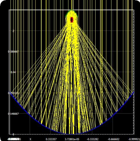
The distribution of heat flux over the absorber tube is essential for heat transfer analysis. Some studies have presented that heat flux distribution over the absorber significantly affects the thermal performance of the PTC receiver [21]. Monte Carlo Ray Tracing method has been used successfully by several authors (Ex. [8, 22]). In the present work, SolTrace software, which uses Monte Carlo Ray Tracing method, is used to calculate the solar flux distribution over the absorber tube. Sun has been modeled as a Gaussian distribution with a cone angle of 2.73 mrad [23]. An ideal tracking system of the PTC system was assumed where the direct normal irradiation was taken as 1000W/m2 for all ray tracing simulations. Both the slope and specularity error of the mirror were considered as 3 mrad. A sample ray tracing in SolTrace is shown in Figure 2. The solar flux distribution obtained from the ray tracing is introduced as a boundary condition in the thermal analysis discussed in the subsequent section.
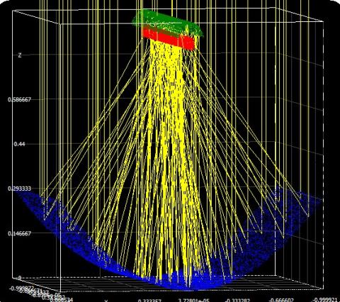
Figure 2. Ray tracing in SolTrace
Simulation conditions are as follows: material of the collector reflector plate is aluminum with reflectivity of 1; shape error is 3 mrad; Specular reflection error is 0.5 mrad. For the secondary reflector, the reflectivity of metal collector tube is of 0.05; shape error is 0.0001mrad; and specular reflection error is 0.0001mrad.
The optical efficiency is calculated as follows:
${{\eta }_{opt}}=\frac{{{q}_{u}}\pi {{D}_{2}}L}{I{{A}_{a}}}$ (2)
where, qu is the surface heat flux of receiver, D2 is the external diameter of receiver tube.
The PTC instantaneous efficiency is calculated as follows:
$\eta =\frac{{{c}_{p}}m({{T}_{out}}-\,{{T}_{in}})}{I{{A}_{a}}}$ (3)
where, Aa is the opening area of parabolic mirror, I is solar radiation intensity, m is the fluid mass flow through the tube, Tin and Tout are the temperatures at the tube inlet and outlet successively.
2.2 Parabolic trough with secondary reflector energy balance
The sunlight incident on the parabolic trough collector (PTC) is focused onto the receiver tube after accounting for the optical losses in the collector (qsolar abs). Some of the sun energy is transferred to the working fluid in the inner tube through convection (qconv absi-HTF). The remaining energy is lost to the atmosphere through convection (qconv,abs). We add a secondary reflector in the aim to minimize losses by radiation (qrad,abo)≈0. The energy balance can be written as follows (see Figure 3):
Figure 3. Configuration and Energy Balance of Parabolic trough collector with secondary reflector system
${{q}_{solarabs}}=\,{{q}_{conv\,abi-HTF}}+{{q}_{cond\,abo-abi}}+{{q}_{conv\,abo}}$ (4)
where, q solar abs is the solar irradiation absorption in the absorber. qconv abi- HTF is the convection heat transfer between the inner absorber wall and the HTF. Q cond abo –abi is the conduction heat transfer through the absorber wall, and q conv abo is the convection heat transfer from the absorber outer to the ambient [24].
2.3 Solar energy absorption
The solar energy absorption on the PTC is calculated using the following equation which is independent of temperature but proportionate to end losses of the collector, intercept factor, width, and length of the parabolic trough [25].
${{Q}_{solarabs}}={{\eta }_{optics}}.I.\theta \left( \phi \right).W..L$ (5)
where, $\eta$optics refers to the optical efficiency; Iin to solar insolation; W and L are the width and length of the collector respectively. The intercept factor ‘$\theta$’ and collector geometrical end losses ‘$\phi$’ are taken as unity.
Fluid flow and heat transfer in both three-dimensional domains, solid and fluid, are described by a system of four equations to be simultaneously solved. This system is presented hereafter [26]:
\(\frac{\partial \rho }{\partial t}+\nabla \left( \rho U \right)=0\) (6)
\(\frac{\partial \left( \rho U \right)}{\partial t}+\nabla .\left( \rho U\otimes U \right)=-\nabla p+\mu \nabla .\nabla U\) (7)
\(\frac{\partial \left( \rho h \right)}{\partial t}+\nabla \left( \rho Uh \right)=\nabla .\left( \lambda \nabla T \right)\) (8)
where, U is the velocity vector, p is the fluid pressure, T is the temperature and h is the enthalpy.
Note that Eq. (8) is applied for both domains fluid and solid.
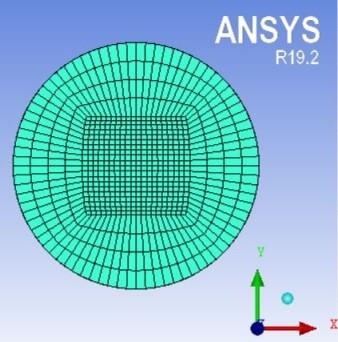
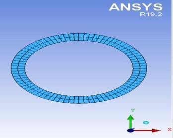
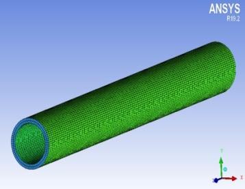
ANSYS ICEM-CFD is used for geometry design and mesh generation. The mesh size and the time step are selected in order to minimize the CPU time and to achieve the desired accuracy. To model a solid-fluid domain, the blocking strategy is used. This technique allows to handle each block separately. This therefore makes it possible to minimize the number of cells. The first block represents the solid domain (tube). In this zone, 101 nodes per unit length are used along the tube and 3 nodes are used along the tube thickness. The second block represents the fluid domain. In this location an O-grid block is used. 21 nodes per unit length are used in both directions x, and y (see Figure 4).
(a)
(b)
(c)
Figure 4. Geometry mesh for solid-fluid domain, (a) fluid mesh (b) and (c) solid mesh
In this work, the materials in question are copper for the tube and Therminol VP-1 for the working fluid. Copper physical properties are predefined in CFX solver. Therminol VP-1 properties (Density, Thermal Conductivity, Heat Capacity and Viscosity) are tabulated in Ref. [27] according to the temperature.
In order to implement fluid properties in the solver we use interpolation functions. Accordingly, these properties are described by the following equations:
$\begin{align} & \rho \ (kg/{{m}^{3}})=-1.587T{{*}^{4}}-4.715T{{*}^{3}}-8.35T{{*}^{2}} \\ & \text{ }-113.6T*+895.1 \\\end{align}$ (9)
$\lambda \ (W/m.K)=-0.002794T{{*}^{2}}-0.02037T*+0.1107$ (10)
$\begin{align} & Cp\ (J/kg.K)=8.152T{{*}^{5}}+11.92T{{*}^{4}}-8.463T{{*}^{3}}- \\ & \text{ }17.87T{{*}^{2}}+383.4T*+2103 \\\end{align}$ (11)
$\begin{align} & \mu \ (Pa.s)=1.995\ \times {{10}^{-6}}\exp (-4.583T*)+3.678\times \\ & \text{ }{{10}^{-4}}\exp (-0.8132T*) \\\end{align}$ (12)
where:
$T*=\left( T(K)-493.0802 \right)/125.2891$ (13)
Note that these expressions are valid only for the temperature range [12 425] °C.
The previous properties equations are implemented in the solver as expressions by using CFX Expression Language (CEL) specific to CFX software.
Before solving the governing equations, domain initialization and boundary conditions must be specified.
The domain is initialized as follows: At time t=0s, we consider that the fluid and the solid are at the same temperature T0; the fluid velocity and pressure are set to zero.
The boundary conditions are applied as follows:
ANSYS CFX is used to solve the mathematical model for solid-fluid domain given by Eqns. (6-8). This software uses a method called element-based finite volume to descritize the conjugate heat transfer and fluid flow equations. The fluid flow is set to turbulent k-ε model with a scalable wall function and the thermal energy model is selected for heat transfer in both domains solid and fluid. The heat flux boundary conditions are introduced using CFX Expression Language (CEL). The advection scheme is set to High resolution and Second order backward Euler method is selected for the transient scheme. The time step is set to 5min, the calculation time is 8hours, and the calculation accuracy is set to 10-4 in terms of Root Mean Square error (RMSE).
This section presents the heat flux and temperature distributions over the absorber tube and collector efficiency at different operating conditions for two cases, circular receiver and semicircular.
8.1 Solar radiation
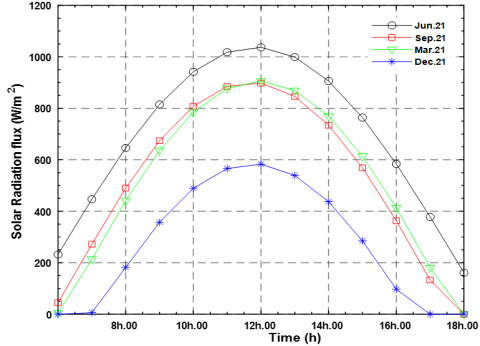
The solar contributions are given for the town of Laghouat. The concentration of solar radiation by using the parabolic trough collector produces high temperature oil. Figure (5) represents the solar radiation as a function of time for 4 days from 4 months.
Figure 5. Variation of modeled solar radiation with time for 4 months in region of Laghouat
The numerical temporal intensity of solar radiation is obtained by using PVSYST5 software for a location (2°56 Longitude and 33°46 Latitude) for 4months during four days: March 21, June 21, September 21 and December 21.
Note that for the day of June 21, the solar radiation is maximal at the real solar noon, which can reach 1037 [w/m²]. The minimal solar radiation, about 600 W/m2, is recorded during the month of December.
8.2 Optical modeling
The main objective of the optical modeling is to determine the concentration of power in the absorber tube, and the evolution of the heat flux at the absorber according to a variation of the incidence angle of rays solar.
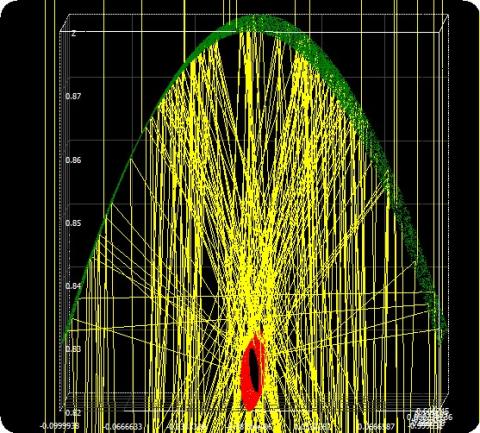
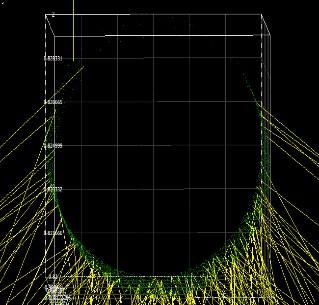
Figure 6. Rays incident on the absorber on the absorber for (a) with secondary reflector (b) without secondary reflector
Figure 6 shows the heat flux distribution on the circumference of absorber tube obtained by ray tracing. The value of heat flux for the case (a) is high on around all the absorber tube due to concentrated of the primary reflector and secondary one. The maximum radiation obtained is about 80000W/m2. A non-linear heat flux distribution is observed over the absorber, which leads to a high temperature gradient.
The value of heat flux for the case (b) is high on the lower portion of the absorber tube due to concentrated solar flux so and low on the upper portion due to direct sunlight for the absorber.
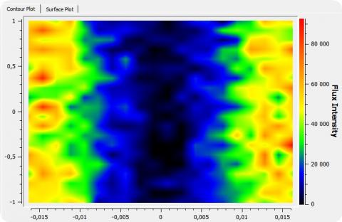
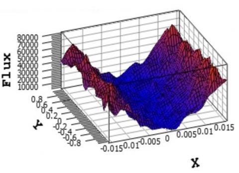
Figures 7 and 8 show consecutively the contour and the surface plot of the average heat flux intensity.
The average heat flux density of receiver is 80000 W/m2, which is numerically simulated using SolTrace software. Simulation model and heat density distribution with the direct normal irradiance of 1000W/m2 were shown in Figure 6. Figure 8 represents a plot paths of ray in the range 1-100 rays. the result of average heat flux density of the collector is 88249W/m2.
Figure 7. Contour plot of heat flux for a parabolic trough collector with secondary reflector on the receiver tube
Figure 8. Surface plot of the heat flux
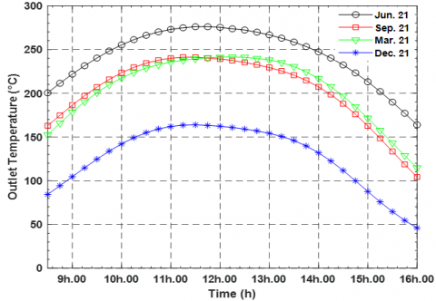
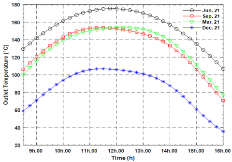
8.3 Fluid outlet temperature
The variations of the temperature, at the tube outlet, during different days are represented in Figure 9 (a) and (b) for both cases: with and without secondary reflector. As it can be seen, the maximum and minimum temperatures are obtained successively during the months of June and December. The fluid temperature at the outlet of the absorber tube is inversely proportional to the direct sunlight, and it mainly depends on the heat quantity absorbed by the tube, which is based on optical and geometric parameters of concentrator. We also notice a difference in maximum temperatures (June) of about 90°C and in minimum temperatures (December) about 50°C between the two cases.
(a)
(b)
Figure 9. Variation of fluid temperature at the tube outlet Versus time, (a) PTC with secondary reflector, (b) PTC without secondary reflector
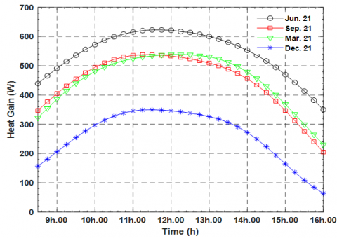
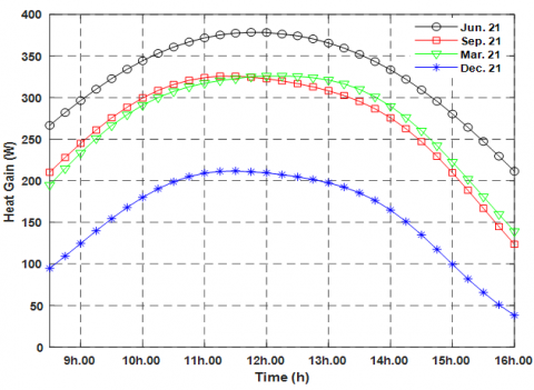
8.4 Useful thermal energy
(a)
(b)
Figure 10. Variation of collected energy with respect to time, (a) PTC with secondary reflector, (b) PTC without secondary reflector
The Therminol VP-1 oil is used as heat carrier fluid. The average mass flow of the fluid through the absorber tube is about 0.005[kg/s], which corresponds to a pressure drop of 0.05 [kPa/m]. During the simulation, the physical properties of the heat carrier fluid are varied depending on the temperature of the fluid according to Eqns. (9) to (13).
Variations of the heat transported by the carrier fluid are shown in Figure 10. We notice that the variation profiles are similar to those of the temperature at the tube outlet. We also note that the difference in heat gain between the two cases (a) and (b) is about 540 W during the month of June and 140 W during the month of December.
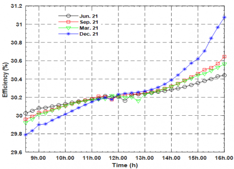
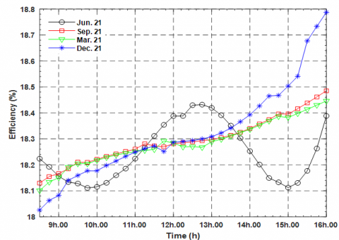
8.5 Thermal efficiency
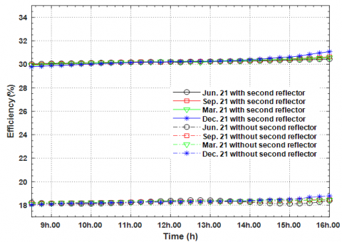
The PTC thermal efficiency values obtained by numerical simulation are reported in Figure 11 (a) and (b). As it can be seen, the efficiency is approximately constant equal to 31% in case (a) for all seasons. For case (b), the efficiency is around 18% for the four seasons. We record then a ratio of 3/2 between the two cases. For a better illustration we have represented the system efficiency for both cases on the same graph (see Figure 12).
(a)
(b)
Figure 11. Variation of instantaneous thermal efficiency Versus time, (a) PTC with secondary reflector, (b) PTC without secondary reflector
Figure 12. PTC efficiency versus time for the two cases, with and without secondary reflector
This paper focuses on the numerical simulation of conjugate heat transfer in the absorber tube of a PTC prototype. In order to determine the system performance, three steps were followed: Firstly, PVSYST5 software is used to provide the numerical temporal intensity of solar radiation for Laghouat city location. Secondly, evolution of the heat flux at the absorber according to a variation of the incidence angle of rays solar is determined by using SolTrace Software. The third step is to simulate the solid-fluid conjugate heat transfer by using ANSYS-CFX solver. Two cases were the subject of the simulation: PTC with and without secondary reflector. Oil Therminol VP-1 is used as a carrier fluid and its physical properties according to temperature are implemented in the solver. The simulation results showed that the maximum fluid temperatures at the outlet of the absorber tube are reached during the month of June while the minimum values are obtained on the month of December. However, the PTC efficiency is constant for the four seasons in both studied cases. Moreover, the calculations showed an increase of the concentration ratio for a PTC when a secondary reflector is used compared to a classical PTC. Indeed, the performance of the system with a second reflector is better than that without a second reflector with a ratio of about 3/2. Another improvement of using a secondary reflector is that the flux around the receiver is distributed more uniformly around the tube.
In the future, further analysis may be considered particularly the optimization of the geometrical and physical parameters of the PTC system.
|
A |
aperture (m) |
|
cp |
specific heat of heat transfer fluid (J kg-1 K-1) |
|
D1 |
absorber tube inner diameter (mm) |
|
D2 |
absorber tube outer diameter (mm) |
|
f |
focal length (m) |
|
I |
solar irradiance (W m-2) |
|
L |
length of receiver tube (m) |
|
m ̇ |
mass flow rate of heat transfer fluid (kg s-1) |
|
T |
temperature (K) |
|
qu |
Heat gain(W) |
|
q |
Heat flux (W/m2) |
|
W |
reflector width (m) |
|
Tin |
inlet temperature of heat transfer fluid (K) |
|
Tout |
outlet temperature of heat transfer fluid (K) |
|
Q |
heat gained by heat transfer fluid (W) |
|
C |
Concentration ratio |
|
$\eta_{\mathrm{opt}}$ |
optical efficiency of collector |
|
P |
Presure(Pa) |
[1] Kalogirou, S.A. (2004). Solar thermal collectors and applications. Progress in Energy and Combustion Science, 30(3): 231-295. https://doi.org/10.1016/j.pecs.2004.02.001
[2] Ouagued, M., Khellaf, A., Loukarfi, L. (2013). Estimation of the temperature, heat gain and heat loss by solar parabolic trough collector under Algerian climate using different thermal oils. Energy Conversion and Management, 75: 191-201. https://doi.org/10.1016/j.enconman.2013.06.011
[3] Cheng, Z.D., He, Y.L., Du, B.C., Wang, K., Qi, L. (2015). Geometric optimization on optical performance of parabolic trough solar collector systems using particles warm optimization algorithm. Applied Energy, 148: 282-293. https://doi.org/10.1016/j.apenergy.2015.03.079
[4] de Risi, A., Milanese, M., Laforgia, D. (2013). Modelling and optimization of transparent parabolic trough collector based on gas-phase nanofluids. Renewable Energy, 58: 134-139. https://doi.org/10.1016/j.renene.2013.03.014
[5] Guenther, M., Michael, J., Simon, C. (2011). Advanced CSP Teaching Materials - Parabolic Trough Technology. Deutsches Zentrum fuer Luft- und Raumfahrt e.V. enerMENA Teaching Materials Implementation Workshop.
[6] Singh, I., Vardhan, S., Singh, S. (2019). A review on solar energy collection for thermal application. International Conference on Current Trends in Engineering, Sciences and Management, At Kuala Lumpur, Malaysia.
[7] Zou, B., Dong, J., Yao, Y., Jiang, Y. (2017). A detailed study on the optical performance of parabolic trough solar collectors with Monte Carlo Ray Tracing method based on theoretical analysis. Sol Energy, 147: 189-201. https://doi.org/10.1016/j.solener.2017.01.055
[8] Xiao, J., He, Y.L., Cheng, Z.D., Tao, Y.B., Xu, R.J. (2009). Performance analysis of parabolic trough solar collector. Journal of Engineering Thermophysics, 30(5): 729-733.
[9] Liang, H., You, S., Zhang, H. (2016). Comparison of three optical models and analysis of geometric parameters for parabolic trough solar collectors. Energy, 96: 37-47. https://doi.org/10.1016/j.energy.2015.12.050
[10] Eck, M., Hirsch, T. (2007). Dynamics and control of parabolic trough collector loops with direct steam generation. Solar Energy, 81(2): 268-279. https://doi.org/10.1016/j.solener.2006.01.008
[11] Pei, G., Li, G.Q., Zhou, X., Ji, J. Su, Y.H. (2012). Experimental study and exergetic analysis of a CPC-type solar water heater system using higher temperature circulation in winter. Solar Energy, 86(5): 1280-1286. https://doi.org/10.1016/j.solener.2012.01.019
[12] Ceylan, I., Ergun, A. (2013). Thermodynamic analysis of a new design of temperature controlled parabolic trough collector. Energy Conversion and Management, 74: 505-510. https://doi.org/10.1016/j.enconman.2013.07.020
[13] Benítez, P., García, R., Miñano, J.C. (1997). Contactless efficient two-stage solar concentrator for tubular absorber. Applied Optics, 36(28): 7119-7124. https://doi.org/10.1364/AO.36.007119
[14] Benítez, P., Miñano, J.C. (1999). Contactless two-stage line focus collectors. J De Physique IV: JP, 9: Pr3-123- Pr123-127. https://doi.org/10.1051/jp4:1999319
[15] Benítez, P., Mohedano Arroyo, R., Miñano , J.C., García R., González, J.C. (1997). Design of CPC-like reflectors within the simultaneous multiple surface design method. In: Proceedings of SPIE, The International Society for Optical Engineering, p. 3139. https://doi.org/10.1117/12.290223
[16] Ries, H., Spirkl, W. (1996). Nonimaging secondary concentrators for large rim angle parabolic troughs with tubular absorbers. Applied Optics, 35(13): 2242-2245. https://doi.org/10.1364/AO.35.002242
[17] Spirkl, W., Ries, H., Muschaweck, J., Timinger, A. (1997). Optimized compact secondary reflectors for parabolic troughs with tubular absorbers. Solar Energy, 61(3): 153-8. https://doi.org/10.1016/S0038-092X(97)00047-9
[18] Wirz, M., Petit, J., Haselbacher, A., Steinfeld, A. (2014). Potential improvements in the optical and thermal efficiencies of parabolic trough concentrators. Solar Energy, 107: 398-414. https://doi.org/10.1016/j.solener.2014.05.002
[19] Canavarro, D., Chaves, J., Collares-Pereira, M. (2013). New second-stage concentrators (XX SMS) for parabolic primaries Comparison with conventional parabolic trough concentrators. Solar Energy, 92: 98-105. https://doi.org/10.1016/j.solener.2013.02.011
[20] Regue, M.H., Benchatti, T., Medjelled, M., Benchatti, A. (2014). Improving the performances of a solar cylindrical parabolic dual refection mirror experimental part. Heat and Technology, 32(1): 171-178.
[21] Li, Z.Y., Huang, Z., Tao, W.Q. (2015). Three-dimensional numerical study on turbulent mixed convection in parabolic trough solar receiver tube. Energy Procedia, 75: 462-466. https://doi.org/10.1016/j.egypro.2015.07.422
[22] Wendelin, T. (2003). SolTRACE: A new optical modeling tool for concentrating. Proceedings of the ASME 2003 International Solar Energy Conference. Solar Energy. Kohala Coast, Hawaii, USA, pp. 253-260. https://doi.org/10.1115/ISEC2003-44090
[23] Aggrey, M., Zhongjie, H., Tunde B.O., Josua P.M. (2016). Influence of optical errors on the thermal and thermodynamic performance of a solar parabolic trough receiver. Solar Energy, 135: 703-718. https://doi.org/10.1016/j.solener.2016.06.045
[24] Lienhard, J.H. (2013). A Heat Transfer Textbook. Courier Corporation.
[25] Duffie, J.A., Beckman, W.A. (1980). Solar Engineering of Thermal Processes. Wiley New York etc.
[26] ANSYS-CFX, Theory Guide. (2019). ANSYS Inc.
[27] Therminol VP-1. Vapor Phase/ Liquid Phase Heat Transfer Fluid (Liquid Phase), Solutia Inc, (2017). http://twt.mpei.ac.ru/tthb/hedh/htf-vp1.pdf/, accessed on Mar. 12, 2018.