Qing Cheng* | Jinpu Jiao
© 2019 IIETA. This article is published by IIETA and is licensed under the CC BY 4.0 license (http://creativecommons.org/licenses/by/4.0/).
OPEN ACCESS
The physical phenomena with fractal features cannot be described by the standard Brownian motion (BM), but by the improved method of fractional Brownian motion (FBM). This paper explores the fractal features of fractional Brownian motion (FBM) and then applies the FBM to interpret the fractal features and fractal scales of gold price fluctuations in China. The results show that the gold price fluctuations in China have obvious, scale-invariant fractal features. Hence, the Chinese gold market is advised to introduce fractal risk management to control the risks. This research widens the applicable scope of the FBM and sheds new light on financial market analysis.
fractional Brownian motion (FBM), fractal features, rescaled range (R/S) analysis, gold price sequence
The theory of Brownian motion (BM), a.k.a. Gaussian process and Wiener process, provides an effective tool to disclose the dynamic features of heat and fluid and to describe the complex evolution of these features. The research and application of the BM features have become a hot topic such fields as thermodynamics, hydrology and water resources. With the continuous improvement of experimental techniques, many fractal features have been observed to deviate from the BM features in such environments as turbulence and the seepage into porous media.
The concept of fractal was proposed by the French-American mathematician Mandelbrot in 1975. It is defined as a physical feature that the components are similar in some way to the whole. Based on the similarity between local and global structures, the law that applies to small time scale could be used in large time scale and vice versa, and this method could also be adopted for predictive research [1].
Fractal features exist widely in thermal phenomena and fluid motions. The fractal is closely correlated with many physical phenomena, such as turbulence, fissure seepage and thermal diffusion. Benzi et al. [2] pointed out that fractal is related to many intermittent phenomena in turbulent diffusion. Benzi et al. [2] held that fissure seepage has fractal features, which bolsters the diffusing capacity of the seepage. Katz and Thompson [3]; Krohn and Thompson [4] discovered the fractal features of pore distribution in sandstone. Heutschel and Procaccia [5] illustrated the energy spectral density [6] of temperature pulsations in open oceans with two power law theories, revealing the fractal features of the energy spectral density. Hurst, British hydrologist and “Father of the Nile”, determined the suitable size of dams based on the fractal features of river flow, and developed the Hurst exponent to measure the persistence of time sequence [7]. Tabeling [8] noticed that the spiral Taylor-Görtler (TG) vortex has fractal features and its fractal dimension increases regularly.
The standard BM obeys the Gaussian (normal) distribution and cannot explain the fractal features of physical phenomena. The BM is highly stochastic, that is, the future data cannot be predicted based on the historical data. Hence, the past motion will not reappear in the future. This calls for a novel means to interpret the fractal features, which are prevalent in thermal phenomena and fluid motions. The fractional Brownian motion (FBM) is a desirable way to explain the fractal features and solve nonlinear problems of the BM [9]. Extended from the classic BM, the FBM has a self-similar, non-stationary independent incremental process, whose mean square displacement (MSD) is a power function of time [10]. Loveioy and Sehertzer [11, 12] relied on the FBM to study hydrological records. Yu et al. [13] employed the FBM to explore the heat transfer process, and noted the nonlinear relationship between the MSD of molecules with time, i.e. the MSD of molecules is proportional to the fractional power of time.
The FBM’s fractal features are mostly measured by the rescaled range (R/S) analysis. The R/S analysis was proposed and refined by Hurst [14-16]. This method reflects the scale invariance of nonlinear statistical features [17], and enjoys a wide range of applications, without needing any assumption. The R/S analysis can explain the long memory and persistence of Non-normal distribution distribution, and provide valuable information for comprehending the complexity of fluid motions. Compared with traditional methods (e.g. autocorrelation function method and power spectrum method), the R/S analysis is suitable for identification and intensity determination of fractal features in non-stationary time sequence.
This paper uses the FBM to analyze fractal features in physical phenomena. The fractal concept, an indicator of the similarities between local and global structures, allows the correlation between the current data and the past data in the time sequence. The results demonstrate the ability of the FBM to interpret the fractal features that the standard BM cannot measure. In addition, this feature of fluid mechanics was applied to economics, expanding the range of applications of the BM. The framework of this paper is as follows. Firstly, the fractal features of the FBM were described, and the advantage of the FBM over the standard BM were enumerated. Next, the R/S analysis was adopted to evaluate the Hurst exponent under the FBM. Finally, numerical examples were cited to prove the broad applicability of the FBM [18, 19].
In 1827, Brown discovered the BM, an irregular random motion, in his study on the movement of pollen. In the BM, the increments in different time intervals are independent of each other, and comply with normal distribution with the mean of zero and the variance of interval length. As mentioned before, the standard BM cannot illustrate the fractal features of physical phenomena, because of the random walk and memoryless data of the BM (i.e. the past data cannot be used to predict the future data).
The FBM is extended from the classic BM by expanding the Hurst exponent from 1/2 to any real number in (0, 1). The FBM has independent incremental process with self-similarity, non-stationarity, whose MSD is a power function of time. Hence, the FBM can interpret the fractal features of physical phenomena [10].
Based on the moving average of Brownian increments, the FBM can be defined as a stochastic process BH(t) satisfying the following condition:
$B_{H}(t)=\frac{1}{\Gamma(H+1 / 2)} \int_{-\infty}^{t} K(t-s)^{H-1 / 2} d B(s)$ (1)
where, H is the Hurst exponent (0<H<1); BH(0)=b0 is a random number; $\Gamma(\cdot)$ is the gamma function; B(s) is the BM; K(t-s) is defined as:
$K(t-s)=\left\{\begin{array}{ll}{(t-s)^{H-1 / 2},} & {0 \leq s \leq t} \\ {(t-s)^{H-1 / 2}-(-s)^{H-1 / 2},} & {s \leq 0}\end{array}\right.$ (2)
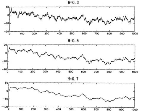
Figure 1. The FBM trajectories at different H values
In the FBM, the increments in different time intervals are not independent of each other but are correlated in different degrees. The correlation varies with the Hurst exponent. If H=1/2, then the FBM is a standard BM and its time increment sequence obeys the normal distribution; if 0<H<1, the sequence property changes with the H value; if 0<H<1/2, the sequence oscillates about the mean; if 1/2<H<1 the sequence is persistent. The FBM trajectories at H=0.3, 0.5 and 0.7 are presented in Figure 1. It can be seen that the greater the H, the steeper the curve, and the weaker the noise. The inverse is also true. Therefore, the Hurst exponent can measure the curve tortuosity.
By its definition, the FBM has the following fractal features:
(1) Statistical self-similarity
The FBM has significant self-similarity, because, for Vγ>0 and t0, the increment of the random process {Xt} of the FBM satisfies:
$\left\{X\left(\left(t_{0}+\tau\right)-X\left(t_{0}\right)\right\}^{d}=\gamma^{-H}\left\{X\left(\left(t_{0}+\gamma \tau\right)-X\left(t_{0}\right)\right\}\right.\right.$ (3)
Self-similarity means that the structures or processes in a system are similar on different spatial or temporal scales. The FBM reflects the self-similar statistical properties of stochastic processes at different time scales, indicating the stability of the dynamic process.
(2) Long-term memory
Long-term memory, a.k.a. long-term correlation, is related to the autocorrelation coefficient of the sequence. The autoco-rrelation function of the FBM increments satisfies:
$C_{H}(\tau)=\frac{\operatorname{Cov}\left\{\Delta B_{H}(t, \tau), \Delta B_{H}(s, \tau)\right\}}{\operatorname{Var}\left[\Delta B_{H}(t, \tau)\right]}$ (4)
where, $\operatorname{Cov}\left[\Delta B_{H}(t, \tau), \Delta B_{H}(s, \tau)\right]$ is the covariance between the FBM increments. This covariance can be expressed as:
$\operatorname{Cov}\left[\Delta B_{H}(t, \tau), \Delta B_{H}(s, \tau)\right]\frac{v_{H}}{2}\left\{|t-s+\tau|^{2 H}+|t-s-\tau|^{2 H}-2|t-s|^{2 H}\right\}$ (5)
The autocorrelation coefficient ρt of the stationary sequence {Xt} decreases slowly at the negative power exponent rate (double curvature) with the growth of the interval order τ [18]:
$\rho_{t} \propto C_{t}^{2 d-1}, \quad \tau \rightarrow \infty$ (6)
where, C is a nonzero constant ensuring the long-term memory of the sequence. According to the definition of the autoco-rrelation coefficient of the FMB increment sequence, the H value depends on the positivity/negativity of the correlation coefficient. If H=1/2, then CH(τ)=0 and the increments are not correlated; if 0<H<1/2, then CH(τ)<0 and the increments are negatively correlated; if 1/2<H<1, then CH(τ)>0 and the increment are positively correlated.
To sum up, in the standard BM, the increments in different time intervals are independent of each other, and comply with normal distribution with the mean of zero and the variance of interval length. The BM is a continuous random walk, its increments are not affected by historical fluctuations, and the same data will not reappear. Thus, the standard BM cannot describe fractal features. By contrast, in the FBM, increments in different time intervals are correlated to different degrees, rather than independent of each other. The correlation varies with the Hurst exponent. Therefore, the structures or processes of the FBM are similar on different spatial or temporal scales, and have fractal features. Thanks to the fractal features, the FBM acts as a useful tool in thermodynamics, fluid mechanics and even economics.
The R/S analysis is a popular non-parametric statistical method, capable of identifying the fractal structure, a structure between stochastic and deterministic structures, from the time sequence. Since its proposal, the R/S analysis has been improved. It is an important way to explore the fractal structure. Without requiring any assumption, the R/S analysis uses the Hurst exponent to determine the fractal structure and state persistence of the time sequence, and outputs stable evaluation results. The R/S analysis can be expressed as:
$(R / S)_{n}=C \cdot n^{H}$ (7)
where, n is the length of the time interval for an increment; C is a constant; H is the Hurst exponent. To estimate the H value, it is necessary to compute the R/S sequence and its time increment sequence, and then perform the regression analysis. The specific steps of the estimation are as follows:
Step 1. Divide the time sequence {Rt} of the length N equally into A non-overlapping, consecutive subsequences Da (a=1,2,…, A), each of which is of the length n (3≤n≤N/2), and denote the elements in each subsequences as Rk,a.
Step 2. Compute the cumulative deviation of each subsequence Da, and record the mean of all subsequence Da as ea.
$X_{k, a}=\sum_{k=1}^{N}\left(R_{k, a}-e_{a}\right)$ (8)
Step 3. Compute the R/S of each subsequence Da, and record the range (difference between the maximum and minimum cumulative deviations) and standard deviation of subsequence Da as Ra and Sa, respectively. Repeat the above process for each subsequence, and obtain a R/S sequence:
$(R / S)_{a}=R_{a} / S_{a}$ (9)
Step 4. Find all subsequence length n (3≤n≤N/2) that are divisible by the sequence length N. Repeat the above steps. Then, evaluate the H value by least squares method according to the following formula:
$\log (R / S)_{n}=\log (C)+H \cdot \log (n)$ (10)
where, log(n) is the explanatory variable; log(R/S) is the explained variable. The coefficient of the explanatory variable is the H value. The R/S analysis can output the most stable results with few or no assumptions. It reveals the intrinsic statistical law of the time sequence, in addition to the nonlinear features. Thus, the R/S analysis has a clear advantage over traditional analysis methods for the time sequence.
There are three possible uses of the R/S analysis. First, the R/S analysis can measure the correlation of the time sequence. If H=1/2, the elements are not correlated; if 0<H<1/2, the elements are negatively correlated; if 1/2<H<1, the elements are positively correlated.
Second, the R/S analysis can determine if the time sequence is stochastic or deterministic. If H=1/2, the time sequence is a stochastic one with independent identically distributed elements, and belongs to the BM (random walk); otherwise, the time sequence is a deterministic one, and belongs to the FBM.
Third, the R/S analysis can judge the persistence of the time sequence after determining the stochasticity/determinacy. If 1/2<H<1, the time sequence enjoys has state persistence, or long-term memory (long-term correlation), i.e. the time sequence maintains the rising/falling trend in the past. Besides, the state persistence is invariant to scale, i.e. state persistence does not change whether the time scale is day or week. The closer the H value is to one, the stronger the persistence of the time sequence. If 0<H<1/2, the time sequence oscillates about the mean value, i.e. the future trend is opposite to the current trend. The closer the H value is to zero, the more significant the oscillation about the mean.
The fractal features of the FBM have been widely adopted to solve many real-world problems: estimating the area of river basin based on river length [8], exploring the viscous fingering of water in clay mud using radial Hele-Shaw cell.
Besides fluid mechanics, the FBM can also solve problems in other fields like the financial sectors. The price fluctuations of financial assets have nonlinearity, long-term memory and fractal features. The fractal features of the FBM can be utilized to solve economic problems. This section adopts the FBM to analyze the fractal features and fractal scale of gold price in China, aiming to expand the application range of the BM.
4.1 Data source
The samples are the daily closing prices (daily prices) and 5-day mean closing prices (weekly prices) of Au99.99 in Shanghai Gold Exchange. Considering data availability, the samples were collected from October 8, 2004 to April 23, 2018, and the missing values were filled up by mean value interpolation.
4.2 Normality test
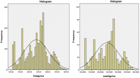
The histogram of the gold price sequence was plotted (Figure 2). Since the density function curve of the histogram differed greatly from that of normal distribution, the gold price sequence does not obey the normal distribution.
Table 1 lists the descriptive statistics of the daily prices and weekly prices of Au99.99 in China. As shown in the table, the skewness was negative and the kurtosis was smaller than 3, indicating that the gold price sequence does not obey normal distribution. Then, the gold price sequence was subjected to Shapiro–Wilk (S-W) test and Kolmogorov–Smirnov (K-S) test, with the original hypothesis that the sequence follows normal distribution. The original hypothesis is proved invalid, for the estimated values were all far greater than 1 %. The distribution of the gold price sequence deviated greatly from normal distribution.
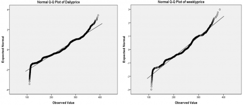
The quantile-quantile (Q-Q) plot was also drawn to verify the normality of the sequence. As shown in Figure 3, the two ends of the sequence both deviated far from the normal distribution, which agrees with the results in Table 1.
In the histogram of the gold price distribution, many price data were concentrated near the mean, and some were scattered in the tails on the left and right sides. Thus, the distribution of gold prices cannot be described accurately by normal distribution. This calls for a new theory to analyze the fluctuations of gold price based on non-normal features.
Figure 2. The histogram of the gold price distribution
Table 1. Statistical analysis of gold price sequence
|
Statistics |
Total number of samples |
Mean |
Standard deviation |
Kurtosis |
Skewness |
S-W statistic |
K-S statistic |
|
Daily prices |
3,327 |
237.08 |
66.09 |
2.83 |
-0.18 |
0.970 |
0.073 |
|
Weekly prices |
714 |
237.13 |
66.13 |
2.29 |
-0.19 |
0.970 |
0.076 |
Figure 3. The Q-Q plot of the gold price distribution
4.3 Empirical analysis on FBM fractal features
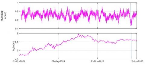
The BM only applies to the time sequence in which the elements are independent of each other and obey normal distribution. By contrast, the FBM can interpret the time sequence data which deviate from the normal distribution. This subsection analyzes the fractal features of gold prices on 2 time scales (daily price and weekly price), and computes the H values of two moving average lengths (60 days and 240 days). The gold prices are shown in log values.
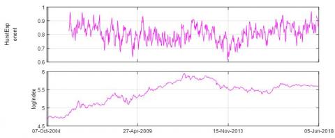
As shown in Figures 4 and 5, the estimated coefficients of H values were around 0.65, much larger than 0.5. This means the daily prices of gold in China have long-term correlations, and carry obvious fractal features. The results echo with the growing trend in gold price trend chart in the medium and long term. In Figure 4, the H value plunged to below 0.5 only at the beginning of 2018, with the moving average length of 60 days, revealing that the daily price of gold will change randomly in the short term. Meanwhile, the H value in the same period in Figure 5 was greater than 0.6, indicating the growing trend of the daily price of gold in the long run.
Figures 6 and 7 show that the daily prices and weekly prices of gold in China had similar H values, i.e. the gold price sequences on the time scale of day and week have the same fractal features. In other words, the gold prices in China is invariant to scale.
Figure 4. The H value of daily prices with the moving average length of 60 days
Figure 5. The H value of daily prices with the moving average length of 240 days
Figure 6. The H value of weekly prices with the moving average length of 60 days
Figure 7. The H value of weekly prices with the moving average length of 240 days
This paper first explores the fractal features of the FBM, and then explores the measurement of the FBM’s fractal measures. Finally, the FBM’s fractal features were applied to explain the sequence of gold prices with similar fluctuation features. This widens the application range and proves the universality of the FBM’s fractal features.
The FBM model can effectively estimate time sequences with fractal features. The FBM not only applies to problems in fluid mechanics and thermodynamics, but also those in fluctuating phenomena with fractal features, such as the capital price fluctuations in economics. In fact, the FBM provides the scientific principle for things with fractal features. The physical phenomena with fractal feature cannot be solved by standard BM, but can be explained by the FBM, an improved version of the BM.
The FBM was introduced to analyze the fractal features of gold price in spot market of China. The analysis achieved a good fitting effect and complemented the traditional market hypothesis. It is confirmed that the gold prices in China have strong fractal features and scale invariance. The gold price sequences on different time scales follow the same or similar statistical laws. If the sequences are assumed to obey normal distribution, the financial investment risk will be underes-timated, and a huge loss may occur. The research on the fractal theory of China’s gold market helps to extract more valuable and accurate risk management information, opens a new way to explore the complexity of China’s gold market, and promises to improve the level of financial risk management.
[1] Mandelbrot, B.B., Wallis, J.R. (1969). Computer experiments with fractional gaussian noises: Part 1, averages and variances. Water Resources Research, 5(1): 242-259.
[2] Benzi, R., Paladin, G., Parisi, G., Vulpiani, A. (1984). On the multifractal nature of fully developed turbulence and chaotic systems. Journal of Physics A: Mathematical and General, 17(18): 3521-3531. http://dx.doi.org/10.1088/0305-4470/17/18/021.
[3] Katz, A.J., Thompson, A.H. (1985). Fractal sandstone pores: Implications for conductivity and pore formation. Physical Review Letters, 54(12): 1325-1328. http://dx.doi.org/10.1103/PhysRevLett.54.1325.
[4] Krohn, C., Thompson, A. (1986). Fractal sandstone pores: Automated measurements using scanning-electron-microscope images. Physical Review B (Condensed Matter), 33(9): 6366-6374. https://doi.org/10.1103/physrevb.33.6366.
[5] Hentschel, H.G.E., Procaccia, I. (1984). Relative diffusion in turbulent media: The fractal dimension of clouds. Physical Review A, 29(3): 1461-1470. http://dx.doi.org/10.1103/PhysRevA.29.1461.
[6] Grant, H.L., Hughes, B.A., Vogel, W.M., Moilliet, A. (1968). The spectrum of temperature fluctuations in turbulent flow. Journal of Fluid Mechanics, 34(3): 423-442. http://dx.doi.org/10.1017/S0022112068001990.
[7] Hack, J.T. (1957). Studies of longitudinal stream profiles in Virginia and Maryland. United States Geological Survey Professional Paper, 294(B): 45-97.
[8] Tabeling, P. (1985). Sudden increase of the fractal dimension in a hydrodynamic system. Physical Review A, 31(5): 3460-3462. https://doi.org/10.1103/physreva.31.3460.
[9] Mondal, M., Biswas, R., Shanchia, K., Hasan, M., Ahmmed, S.F. (2019). Numerical investigation with stability convergence analysis of chemically hydromagnetic Casson nanofluid flow in the effects of thermophoresis and Brownian motion, International Journal of Heat and Technology, 37(1): 59-70. https://doi.org/10.18280/ijht.370107.
[10] Mandelbrot, B.B., Ness, J.W.V. (1968). Fractional brownian motions, fractional noises and applications. Siam Review, 10(4): 422-437. http://dx.doi.org/10.1137/1010093.
[11] Lovejoy, S., Schertzer, D. (1985). Generalized scale invariance in the atmosphere and fractal models of rain. Water Resources Research, 21(8): 1233-1250. http://dx.doi.org/10.1029/WR021i008p01233.
[12] Lovejoy, S., Schertzer, D. (1986). Scale invariance, symmetries, fractals, and stochastic simulations of atmospheric phenomena. Bulletin of the American Meteorological Society, 67(1): 21-32.
[13] Yu, Z., Shao, X., Wachs, A. (2006). A fictitious domain method for particulate flows with heat transfer. Journal of Computational Physics, 217: 424-452. http://dx.doi.org/10.1016/S1001-6058(06)60098-X.
[14] Mandelbrot, B.B. (1972). Statistical methodology for non-periodic cycles: From the covariance to R/S analysis. Annals of Economic and Social Measurement, 1(3): 255-290. http://ideas.repec.org/h/nbr/nberch/9433.html.
[15] Mandelbrot, B.B., Wheeler, J.A. (1998). The fractal geometry of nature. American Journal of Physics, 51(4): 468.
[16] Lo, A.W. (1991). Long-term memory in stock market prices. Econometrica, 59(5): 1279-1313. https://www.jstor.org/stable/2938368.
[17] He, K.Q., Sun, L.N., Wang, S.J. (2009). Displacement fractal parameter Hurst index and its application to prediction of debris landslides. Chinese Journal of Rock Mechanics and Engineering, 28(6): 1107-1115. http://dx.chinadoi.cn/10.3321/j.issn:1000-6915.2009.06. 004
[18] Bărbulescu, A., Serban, C., Maftei, C. (2010). Evaluation of Hurst exponent for precipitation time series. Proceedings of the 14th WSEAS international conference on Computers: part of the 14th WSEAS CSCC multiconference - Volume II. World Scientific and Engineering Academy and Society (WSEAS).
[19] Araújo, M.B., Pearson, R.G., Thuiller, W., Erhard, M. (2005). Validation of species–climate impact models under climate change. Global Change Biology, 11(9): 1504-1513. https://doi.org/10.1111/j.1365-2486.2005.01000.x