Nguyen Ngoc Nam | Sang-Do Lee | Sam-Sang You* | Bui Duc Hong Phuc
© 2019 IIETA. This article is published by IIETA and is licensed under the CC BY 4.0 license (http://creativecommons.org/licenses/by/4.0/).
OPEN ACCESS
The purpose of this study is to investigate dynamical behaviors and active control synthesis of mass flowrate in the flow boiling of microchannel, which provides the inspiration to effective pressure drop treatments under parameter variations, exogenous disturbances, and measurement noises. The nonlinear mathematical model has been established through the momentum balance of surge tank and boiling microchannel. The pressure drop oscillations are one of the most severe dynamical instabilities for the boiling two-phase flow microchannel system under various uncertainties and disturbances, certainly leading to thermal and mechanical fatigues and breakage with excessive wear on the microchannel constituents. The boiling microchannel system exhibits complex dynamical behaviors; periodic, quasi-periodic, and chaotic behaviors. Those behaviors are characterized by using phase portrait, bifurcation diagram, and time series analysis. Based on Jacobian linearization around the equilibrium points, the dynamical system can be expressed in the state-space representation with parametric uncertainty. Through this study, it was found that the robust control synthesis can cope with flow oscillations as well as flow instability in an uncertain microchannel system. The extensive simulation results indicate that the proposed control scheme has offered robust performances and stability of the microchannel system under various uncertainties.
two-phase flow, boiling microchannel, pressure drop, flow instability,bifurcation, robust control
The high flux heat removal for microchannel is one of challenging heat sink schemes with ever-increasing demands in the thermal management of high-power density electronics or advanced electronic components [1]. Moreover, two–phase flow instabilities can take place in nuclear power reactors, cryogenic and chemical processes and high heat flux electronic devices. In general, boiling and cooling technologies are increasingly being utilized for various applications in the fields of military, space, and automation. In the practical electronic devices, the heat loads could exceed 1000 W/cm2 while the surface temperature of chips and devices needs to maintain below 85oC for safe operations [2, 3]. Microchannel flow boiling is an advanced cooling method which guarantees high thermal performance [4]. In addition, many efforts have been made to design microchannel heat exchangers to maximize the heat transfer with minimal pump demand [2, 3, 5].
In recent years, several investigators have shown that boiling microchannel becomes very popular scheme in harnessing latent heat of vaporization with high heat flux dissipation [2-4]. It is known that the mini/microchannel system can significantly enhance the convective heat transfer rates for flow boiling in microscale heat sinks. When two-phase flow occurs in microchannels, boiling flows are prone to severe dynamic instabilities and fluctuations, such as oscillations in mass flowrates, pressure drops, and temperatures. These dynamic oscillations are undesirable because they can cause severe structure vibrations and can make it difficult to ensure smooth operations for microchannel system. The microchannel surface may dry out and subsequently leads to hot pots and eventually device failures due to disturb the heat transfer. In the real system, the mass flowrate characteristics are closely related to transient dry out and potential local overheating and burnout of the system, and these should be efficiently prevented by optimal thermal management.
It is crucial to understand and predict onset of boiling and flow instabilities in the active thermal management, especially for the designs and operations of microchannel system. The pressure drop oscillation occurs where the mass flowrate operates in the two-phase negative-slope region for flow boiling. Therefore, the microchannel system must have an upstream compressible volume to decrease the pressure drops and increase the mass flowrates in the negative-slope flow. The compressible volume exits in long test sections or can be artificially introduced by placing the surge tank upstream of the heated channel section. In microchannel, the ratio of length and diameter (L/d>150) is easily attained, and many studies have been carried out on boiling by observing flow oscillations in the heated channel [6].
Although there have been several studies on the flow instabilities in the mini/microchannel system, most existing researches focus on removing the heat flux at the device and analyzing oscillations of the pressure drop and mass flowrate [1-3, 6]. Active suppression or management of dynamic oscillation has not received much attention especially. How to manage the flow boiling instabilities gives inspiration to many researchers for active control synthesis. Recently, some methods have been applied to suppress dynamic oscillations using the inlet restrictor [7], in which the limited capability for power pump was proposed since relatively large pressure drops must be sustained due to the restrictor; a set of active control schemes were proposed to deal with dynamic oscillations in mass flowrates and pressure drops using state feedback [8, 9]. However, there has been no research report on robust control synthesis that simultaneously deals with model uncertainty, exogenous disturbances and measurement noises in the microchannel system.
The rest of this paper is organized as follows. Section 2 introduces the mathematical model of boiling microchannel system obtained by considering dynamic interactions between surge tank and boiling channel. Next, the nonlinear analysis has been performed to describe the dynamic behaviors for flow boiling in Section 3. In Section 4, the active controller has been applied to suppress the flow instability in microchannel system. The simulation results and discussion are presented in Section 5. The numerical tests demonstrate that robust performance and stability are guaranteed under parametric variations, external disturbances, and sensor noises. Finally, the conclusions will be drawn in Section 6.
Figure 1 shows a schematic diagram of the heated horizontal microchannel system. The complete system includes a feeder section, a heated tube section, and a fluid recovery unit. The input section consists of a water tank, a pump, a valve 1, a valve 2 and a filter. The fluid supply into the boiling channel can be achieved through the valve 1 and the pump which typically would adjust the mass flowrate of the working fluid. The boiling channel can be protected against water damage by the relief valve 2 which allows the fluid flows back to a large reservoir of water tank if the channel pressure is too high. The heated section consists of a surge tank, a horizontal heated tube, and a valve 3 along with a flow meter and pressure meters, in which two-phase flow instabilities may occur under flow supply conditions. The surge tank is utilized in the tube inlet to ensure an upstream compressible volume. The pressure meters are installed at the both sides of the heated tube for measuring differential pressures. For the fluid recovery, the two-phase flows in the heated tube enter towards condenser directly. Then the condenser maintains a constant exit pressure as for the heated section.
Figure 1. Schematic diagram of boiling microchannel system
In order to build the mathematical model, some assumptions are made as follows:
For the two-phase flow in a horizontal channel, the lumped one-dimension momentum balance equations for the upstream surge tank and the boiling channel can be respectively written as follows:
${{\tilde{P}}_{in}}-{{\tilde{P}}_{I}}={{J}_{I}}\frac{d{{{\dot{m}}}_{I}}}{dt},{{J}_{I}}=\sum\limits_{i}{\frac{{{{\tilde{A}}}_{i}}}{{{L}_{i}}}}$ (1)
${{\tilde{P}}_{in}}-{{\tilde{P}}_{out}}=\Delta {{\tilde{P}}_{tp}}+J\frac{d\dot{m}}{dt}, J=\sum{\frac{{\tilde{A}}}{L}}$ (2)
where ${{P}_{in}}$, ${{P}_{out}}$, ${{P}_{I}}$, $\Delta {{P}_{tp}}$, ${{J}_{I}}$, $J$, ${{\dot{m}}_{I}}$, $\dot{m}$, ${{A}_{i}}$, $A$, ${{L}_{i}}$, $L$ are pressure input, pressure output, pressure into /out of the surge tank, pressure drop across in boiling section, inertia into / out of the surge tank, inertia into the boiling section, mass flowrate into/ out of the surge tank, mass flowrate into the boiling section, areas across the surge tank, areas across the boiling section, lengths in the surge tank, length in boiling section, respectively.
Let ${{\dot{m}}_{1}}$ and ${{\dot{m}}_{2}}$ denote the mass flowrates of saturated vapor and saturated liquid, respectively. The pressure loss of two-phase liquid-vapor mixture in the microchannel can be written as
$\frac{d\Delta {{P}_{tp}}}{d\dot{m}}=\alpha (\dot{m}-{{\dot{m}}_{1}})(\dot{m}-{{\dot{m}}_{2}})$ (3)
where $\alpha $ is a positive constant. Taking time derivative of Eqs. (1) and (2) yields, respectively
$\left\{ \begin{align} & \frac{d{{P}_{in}}}{dt}-\frac{d{{P}_{I}}}{dt}={{J}_{I}}\frac{{{d}^{2}}{{{\dot{m}}}_{I}}}{d{{t}^{2}}} \\ & \frac{d{{P}_{in}}}{dt}=\frac{d\Delta {{P}_{tp}}}{d\dot{m}}\frac{d\dot{m}}{dt}+J\frac{{{d}^{2}}\dot{m}}{d{{t}^{2}}} \\\end{align} \right.$ (4)
The overall mass flowrate at inlet is given by ${{\dot{m}}_{0}}=\dot{m}+{{\dot{m}}_{I}}$ using the mass balance, in which $\dot{m}$ is the mass flowrate into the boiling channel, and ${{\dot{m}}_{I}}$ is the mass flowrate into or out of the surge tank. A set of differential equations for the overall mass flowrates can be obtained by
$\frac{d{{{\dot{m}}}_{0}}}{dt}=\frac{d\dot{m}}{dt}+\frac{d{{{\dot{m}}}_{I}}}{dt}, \frac{{{d}^{2}}{{{\dot{m}}}_{0}}}{d{{t}^{2}}}=\frac{{{d}^{2}}\dot{m}}{d{{t}^{2}}}+\frac{{{d}^{2}}{{{\dot{m}}}_{I}}}{d{{t}^{2}}}$ (5)
In this study, the gas is assumed to be inert and polytrophic in the tank. The parameter k is a fixed polytrophic index of expansion. The relation between pressure PI and gas volume VI can be represented by
${{P}_{I}}V_{I}^{k}=\text{constant}$ (6)
Differentiating Eq. (6) leads to
$\frac{d{{P}_{I}}}{dt}=-\frac{k{{P}_{I}}}{{{V}_{I}}}\frac{d{{V}_{I}}}{dt}$ (7)
The mass flowrate into and out of the compressible gas in the surge tank will be in proportion to the upstream liquid with a density ${{\rho }_{f}}$, and then it leads to
${{\dot{m}}_{I}}=-{{\rho }_{f}}\frac{d{{V}_{I}}}{dt}$, $\frac{d{{V}_{I}}}{dt}=-\frac{{{{\dot{m}}}_{I}}}{{{\rho }_{f}}}$ (8)
Substituting Eq. (8) into Eq. (7) can be described by
$\frac{d{{P}_{I}}}{dt}=\frac{k{{P}_{I}}}{{{\rho }_{f}}{{V}_{I}}}{{\dot{m}}_{I}}$ (9)
In particular, the mass flowrate is assumed to be constant. Substituting Eqs. (3), (5) and (9) into Eq. (4) yields
$\frac{{{d}^{2}}\dot{m}}{d{{t}^{2}}}+(a{{\dot{m}}^{2}}-b\dot{m}+c)\frac{d\dot{m}}{dt}+d.\dot{m}=d.{{\dot{m}}_{0}}$ (10)
where $a=\frac{\alpha }{\left( {{J}_{I}}+J \right)}$, $b=\frac{\alpha }{\left( {{J}_{I}}+J \right)}\left( {{{\dot{m}}}_{1}}+{{{\dot{m}}}_{2}} \right)\dot{m}$, $c=\frac{\alpha }{\left( {{J}_{I}}+J \right)}{{\dot{m}}_{1}}{{\dot{m}}_{2}}_{2}$, $d=\frac{1}{\left( {{J}_{I}}+J \right)}\frac{k{{{\tilde{P}}}_{I}}}{{{\rho }_{f}}{{V}_{I}}}$.
The pressure drop in the boiling channel is described by
$\frac{d\Delta {{{\tilde{P}}}_{tp}}}{d\dot{m}}=\alpha (\dot{m}-{{\dot{m}}_{1}})(\dot{m}-{{\dot{m}}_{2}})=\left( {{J}_{I}}+J \right)(a{{\dot{m}}^{2}}-b\dot{m}+c)$ (11)
By integrating Eq. (11) over $\dot{m}$, the pressure drop of the boiling flowrate across the channel is given by
$\Delta {{\tilde{P}}_{tp}}=\left( {{J}_{I}}+J \right)(\frac{a}{3}{{\dot{m}}^{3}}-\frac{b}{2}{{\dot{m}}^{2}}+c\dot{m}+\gamma )$ (12)
The mathematical formulation can be described in the state-space representation to characterize the nonlinear behaviors. Base on the equilibrium points the vector field could be utilized for dynamical analysis. The bifurcation analysis will be taken into account to evaluate various parameter changes on the stability of two-phase flow.
3.1 Local dynamical analysis
To obtain a state-space model, the state variables are defined as follows: ${{x}_{1}}=\dot{m}$ and ${{x}_{2}}=\frac{d\dot{m}}{dt}$. Then the dynamical model described in Eq. (10) is given by
$\left\{ \begin{align} & \left[ \begin{matrix} {{{\dot{x}}}_{1}} \\ {{{\dot{x}}}_{2}} \\\end{matrix} \right]=\left[ \begin{matrix} {{x}_{2}} \\ -\left( ax_{1}^{2}-b{{x}_{1}}+c \right){{x}_{2}}-d{{x}_{1}}+d{{m}_{0}} \\\end{matrix} \right] \\ & y=\left[ \begin{matrix} 1 & 0 \\\end{matrix} \right]\left[ \begin{matrix} {{x}_{1}} \\ {{x}_{2}} \\\end{matrix} \right] \\\end{align} \right.$ (13)
where x1 is a mass flowrate, x2 is a rate of the mass flowrate, and y is the vector of system output. Then the equilibrium points (EQ) can be obtained as follows: $EQ=\left\{ {{Q}_{1}}({{x}_{11}},0);{{Q}_{2}}({{x}_{12}},0;...{{Q}_{n}}({{x}_{1n}},0) \right\}$. In this model, the microchannel system has a unique equilibrium point, $Q=({{m}_{0}},0)$ for all parameter values. To determine the local stability around equilibrium points, the microchannel model can be linearized, using the Jacobian matrix A , as follows
$A={{\left[ \begin{matrix} 0 & 1 \\ -\left( 2a{{x}_{1}}-b \right){{x}_{2}}-d & -ax_{1}^{2}+b{{x}_{1}}-c \\\end{matrix} \right]}_{Q}}$ (14)
The characteristic equation for the eigenvalues $\lambda$ at the equilibrium point is described by
${{\lambda }^{2}}+{{\beta }_{1}}\lambda +{{\beta }_{2}}=0$ (15)
where ${{\beta }_{1}}=am_{0}^{2}-b{{m}_{0}}+c$ and ${{\beta }_{2}}=d$. For the asymptotic stability, the necessary and sufficient conditions for ensuring all eigenvalues of negative real parts are: ${{\beta }_{1}}>0$ and ${{\beta }_{1}}{{\beta }_{2}}>0$.
Table 1. Boiling microchannel parameters
|
Parameters |
Values |
Unit |
|
Channel with (W) |
61 |
$\mu m$ |
|
Channel height (H) |
272 |
$\mu m$ |
|
Channel length (L) |
15 |
$mm$ |
|
Hydraulic (Dh) |
100 |
$\mu m$ |
|
Effective cross-section area (Across) |
1.66 |
$m{{m}^{2}}$ |
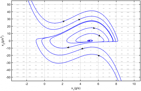
The nominal parameters values of the boiling microchannel is shown in Table 1, and some coefficients of the boiling microchannel system are calculated as $a=1.4283$, $b=1.6163$, $c=-14.4716$, and $d=1.0028$[9]. Two-phase flow behaviors of boiling microchannel can be depicted using the phase plane or vector field analysis. The phase portrait for the boiling microchannel in case of ${{\beta }_{1}}>0$, and ${{\beta }_{1}}{{\beta }_{2}}<0$ is shown in Figure 2. In case of ${{m}_{0}}=5$, at the equilibrium point $Q=(5,0)$, one of the real parts of both eigenvalues is positive. According to the Routh-Hurwitz’s theorem, there exists the flow instability, in which the trajectory diverges away from the equilibrium. Moreover, all the neighboring trajectories converge to the limit cycle from both sides (interior and exterior) as time approaches infinity. Note that the image of a periodic solution in the phase portrait is a closed trajectory, calling periodic orbit or closed orbit. On the phase plane, a limit cycle is defined as an isolated closed orbit. This closed trajectory describes the isolated periodic behaviors of the system, and any perturbation from the closed orbit causes the system trajectory to return to it, making the system response stick to the stable limit cycle.
Figure 2. Phase portraits of the boiling microchannel system for the parameter value of ${{m}_{0}}=5$.
The dynamic behavior due to increasing the mass flowrate ${{m}_{0}}$ is shown in Figure 3. In the case of ${{m}_{0}}=0.9%$, at the equilibrium point $Q=(9,0)$, the real parts of both eigenvalues are negative from the conditions $β_1>0$ and $β_1β_2>0$. According to the Routh-Hurwitz's criterion, the dynamic behaviour of boiling microchannel system is stable, and all trajectories converge to the stable equilibrium point with different initial conditions.
Figure 3. Phase portraits of the microchannel system for the parameter value of ${{m}_{0}}=9$
Figure 4. Mass flowrate oscillation in the boiling channel for the parameter value of ${{m}_{0}}=5$
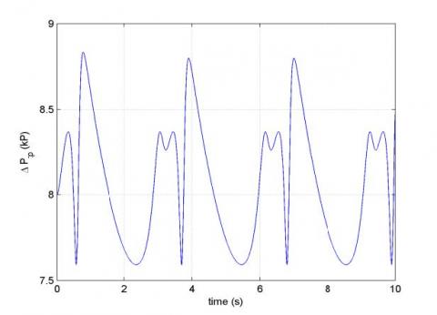
Figure 5. Pressure drop oscillation in boiling channel for the parameter value of ${{m}_{0}}=5$
Figs. 4 and 5 show the time histories of mass flowrates and pressure drops in boiling microchannel at a volume flowrate of 5 g/s with the constant heat flux. It can be observed that the mass flowrate and the pressure drop exhibit a limit cycle behavior with constant amplitude and time period.
3.2 Bifurcation analysis
Referring to Eq. (14), the input parameters are given in Table 1. Specifically, ${m}_{0}$ is selected as a bifurcation parameter. From the characteristic polynomials in Eq. (15),
${{\lambda }_{1}},{{\lambda }_{2}}=-0.5({{m}_{0}}-1.389)({{m}_{0}}-5.276)\pm 0.5\sqrt{{{\left( 1.5m_{0}^{2}-10{{m}_{0}}+11 \right)}^{2}}-40}$
It is noted that the eigenvalue formula has specific dynamic characteristics for ${{m}_{0}}=1.389$, and ${{m}_{0}}=5.276$. A local bifurcation occurs when a parameter change causes the stability of an equilibrium point to change.
Table 2. Stability classifications for bifurcation parameter
|
Parameter |
Eigenvalue |
Stability |
|
${{m}_{0}}<1.389$ |
negative real |
stable |
|
$1.389<{{m}_{0}}<5.276$ |
positive real |
unstable |
|
${{m}_{0}}>5.2764 |
negative real |
stable |
As shown in Table 2, the boiling microchannel system has two bifurcation points at ${{m}_{0}}=1.389$ and ${{m}_{0}}=5.276$, where the system has phase changes: stable node to unstable and unstable to stable node.
Figure 6 depicts the pressure drops of two-phase flow section. At two special points of ${{A}_{1}}$ and ${{A}_{2}}$, Phase changes are occuring; at ${{A}_{1}}$, phase change from superheated to two-phase flow and vice-versa with ${{m}_{0}}=1.389$; at ${{A}_{2}}$, phase change from two-phase to subcooled and vice-versa with ${{m}_{0}}=5.276$. Thus, the microchannel system with zero slopes is bifurcating.
Figure 6. Phase portraits for pressure drop in case of parameter value ${{m}_{0}}=5$
Figure 7 shows the bifurcation diagram with control parameter change of the mass flowrate. In the case of ${{m}_{0}}<1.389$, the eigenvalue is negative, and the pressure drop is stable (superheated). In case of ${{m}_{0}}=1.389$ with ${{\lambda }_{1,2}}=\pm j3.16228$, the eigenvalues are obtained as two conjugates with no real part, and then a Hopf bifurcation occurs. In the case of $1.389<{{m}_{0}}<5.2769$, the system is unstable with positive characteristic eigenvalues. In the case of ${{m}_{0}}=5.2769$ with ${{\lambda }_{1,2}}=\pm j3.16228$, Hopf bifurcation occurs again. In the case of ${{m}_{0}}>5.2769$, since the eigenvalues have negative real parts, then the pressure drop is stable (subcooled).
The bifurcation diagrams at ${{A}_{1}}$ and ${{A}_{2}}$ are shown in Figures 8 and 9, which completely describe dynamical behaviors for two state variables $\dot{m}$, and $\dot{m}/dt$ as the control parameter $a$. In case of mass flowrate ${{m}_{0}}=1.389$ with parameter $a=1.4283$, the bifurcation at ${{A}_{1}}$ occurs and the qualitative behavior around ${{A}_{1}}$ is center. On decreasing bifurcation parameter $a$, two state variables are oscillating as illustrated in Figure 8. In case of ${{m}_{0}}=5.2769$ with $a=1.4283$, the bifurcation at ${{A}_{2}}$ occurs and the qualitative behavior around ${{A}_{2}}$ is center. As shown in Figure 9, two state variables are now oscillating with changing control parameter $a$.
Figure 7. Bifurcation diagram with changing parameter ${{m}_{0}}=0$
Figure 8. Bifurcation diagram at ${{A}_{1}}$ when $a$ is bifurcation parameter
Figure 9. Bifurcation diagram at ${{A}_{2}}$ when $a$ is bifurcation parameter
4.1 Model linearization
The dynamic behaviors of the microchannel around equilibrium points have been described by depending on the flowrate supply. Instead of directly controlling a nonlinear system, the flow boiling system can be linearized in the vicinity of equilibrium points to utilize a linear control theory.
Consider the state-space representations for nonlinear and linear version given as follows:
$\left\{ \begin{matrix} \dot{x}(t)=f(x(t),u(t))\approx Ax(t)+Bu(t) \\ y(t)=h(x(t),u(t))\approx Cx(t)+Du(t) \\\end{matrix}\right.$ (17)
where $x(t)$ is the state variable vector, $y(t)$ is the system output, $u(t)$ is the control input; $f(x,u)$ and $h(x,u)$ are continuously differential functions given in Eq. (13). Note that the microchannel system has the equilibrium point at $Q({{x}_{1}},{{x}_{2}})=({{m}_{0}},0)$. By computing Jacobian linearization of Eq. (17), the state space matrices are obtained as follows:
$A={{\left. \frac{\partial f}{\partial x} \right|}_{Q}}=\left[ \begin{matrix} 0 & 1 \\ -d & -(am_{0}^{2}-b{{m}_{0}}+c) \\\end{matrix} \right]$;
$B={{\left. \frac{\partial f}{\partial u} \right|}_{Q}}=\left[ \begin{matrix} 0 \\ d \\\end{matrix} \right]$;
$C={{\left. \frac{\partial h}{\partial x} \right|}_{Q}}=\left[ \begin{matrix} 1 & 0 \\\end{matrix} \right]$;
$D={{\left. \frac{\partial h}{\partial u} \right|}_{Q}}=\left[ 0 \right]$
Using the state space matrices $(A,B,C,D)$, the open-loop transfer function corresponding to the microchannel model can be described as follows:
$\begin{align} & G(s)=\left[ \frac{\left. A \right|}{\left. C \right|}\frac{B}{D} \right]=C{{(sI-A)}^{-1}}B+D \\ & \text{ }=\frac{d}{{{s}^{2}}+(m_{0}^{2}a-{{m}_{0}}b+c)s+d} \\\end{align}$ (18)
4.2 Uncertainty model
Robust control synthesis will begin with model uncertainty or model perturbation. In general, the system uncertainty includes the parameter variations, the external disturbances and sensor/actual noises. Moreover, a mathematical model of any real system is just an approximation of the physical system dynamics, or considering low-frequency dynamics. The unstructured uncertainty is useful for describing unmodelled or neglected high-frequency dynamics. In the microchannel, the parameter uncertainty can be lumped into ${{\Delta }_{m}}$ which may be expressed in an input multiplicative form, as shown in Figure 10.
Figure 10. Uncertain dynamic model with input multiplicative representation
The robust control problem is to stabilize a set of perturbed plant $(\prod )$ given as follows [10, 11]:
$\prod :\ {{G}_{P}}(s)=G(s)\left( I+{{\Delta }_{m}}(s){{W}_{m}}(s) \right);\underbrace{\left( \left| {{\Delta }_{m}}(j\omega ) \right|\le 1 \right),\forall \omega }_{{{\left\| {{\Delta }_{m}} \right\|}_{\infty }}\le 1}$ (19)
where $G(s)$, and ${{G}_{p}}(s)$ represent nominal and perturbed model, respectively; ${{W}_{m}}$ is the uncertainty weighting function, and ${{\Delta }_{m}}(s)$ is a normalized value satisfying ${{\left\| {{\Delta }_{M}}(j\omega ) \right\|}_{\infty }}\le 1$. Further, the set of dynamic models with parametric uncertainty can be represented as follows:
${{G}_{P}}(s)=\left[ \frac{\left. A+\sum _{i=1}^{k}{{\alpha }_{i}}{{A}_{i}} \right|}{\left. C+\sum _{i=1}^{k}{{\alpha }_{i}}{{C}_{i}} \right|}\frac{B+\sum _{i=1}^{k}{{\alpha }_{i}}{{B}_{i}}}{D+\sum _{i=1}^{k}{{\alpha }_{i}}{{D}_{i}}} \right]$ (20)
where the system matrices $(A,B,C,D)$ represent the nominal model, and ${{\alpha }_{i}}{{A}_{i}}$ is the parameter uncertainty. The perturbed plant with uncertainty has a boundary of ${{l}_{m}}(j\omega )$ at each angular frequency ($\omega\in R$). This boundary includes all possible plant ${{G}_{P}}(s)\in \prod $ defined by
${{l}_{m}}(\omega )=\underset{{{G}_{p}}\in \Pi }{\mathop{\max }}\,\left| \frac{{{G}_{p}}(j\omega )-G(j\omega )}{G(j\omega )} \right|$ (21)
Then the weighting function ${{W}_{m}}(s)$ is chosen to cover the boundary ${{l}_{m}}(j\omega )$ as follows:
$\left| {{W}_{m}}(j\omega ) \right|\ge {{l}_{m}},\forall \omega $ (22)
4.3 Control synthesis
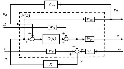
Based on the linear control theory [10], the robust ${{H}_{\infty }}$ controller has proven to be the most effective approach in dealing with the complex dynamical systems affected by the uncertainties, disturbances, and noises. In order to analyze and synthesize the control system for the robustness and stability, the generalized plant $P(s)$ should include all weighting functions affecting the microchannel system dynamics, as shown in Figure 11.
Figure 11. Overall control structure with the generalized plant
For the general block diagram of the plant $P$ with perturbation $Δ_m$, a weighting function $w_p$ is added to describe the performance requirement. The reference input $r$ represents the set point that the system output should follow. The robust controller can make the regulated response $z$ exactly follow the input reference $r$ against uncertainties. To check the robustness issue, the exogenous disturbance $d$ as well as the sensor noise $n$ would be considered in the complete control system. Noting that all weighting functions include disturbances ${{w}_{d}}$, noises ${{w}_{n}}$, and references ${{w}_{r}}$, the generalized control system can be written as
$\left[ \begin{matrix} {{y}_{\Delta }} \\ \underset{---}{\mathop{z}}\, \\ y \\\end{matrix} \right]=\underbrace{\left[ \begin{matrix} 0 & 0 & 0 & 0 & {{w}_{m}} \\ {{w}_{p}}G & {{w}_{p}}{{w}_{d}} & 0 & 0 & {{w}_{p}}G \\ -G & -{{w}_{d}} & {{w}_{r}} & -{{w}_{n}} & -G \\\end{matrix} \right]}_{P(s)}\left[ \begin{matrix} \begin{matrix} {{u}_{\Delta }} \\ d \\ r \\ \underset{---}{\mathop{n}}\, \\\end{matrix} \\ u \\\end{matrix} \right],P=\left[ \begin{matrix} {{P}_{11}} & {{P}_{12}} \\ {{P}_{21}} & {{P}_{22}} \\\end{matrix} \right]$ (23)
where ${{u}_{\Delta }}$ and ${{y}_{\Delta }}$ describe the input and output signals to uncertainty block ${{\Delta }_{m}}$.
Figure 12. Feedback interconnection for control synthesis and analysis
As illustrated in Figures 11 and 12, the $N-{{\Delta }_{m}}$ structure can be created by grouping the generalized plant $P(s)$ and controller $K(s)$. In order to utilize the robust control synthesis, the closed-loop transfer matrix $N(s)$ connects the generalized plant $P$ with the controller $K$ via a lower linear fractional transformation (LLFT), and it is defined by
$\left[ \begin{matrix} {{y}_{\Delta }} \\ z \\\end{matrix} \right]=N\left[ \begin{matrix} {{u}_{\Delta }} \\ w \\\end{matrix} \right]$ (24)
where $w={{\left[ \begin{matrix} d & n & r \\\end{matrix} \right]}^{T}}$ and $z=N.w$. The transfer function matrix N is specifically calculated as
$N={{F}_{LLFT}}\left( P,K \right)={{P}_{11}}+{{P}_{12}}K{{\left( I-{{P}_{22}}K \right)}^{-1}}{{P}_{21}}=\left[ \begin{matrix} {{N}_{11}} & {{N}_{12}} \\ {{N}_{21}} & {{N}_{22}} \\\end{matrix} \right]$ (25)
where ${{N}_{11}}=\left[ {{W}_{m}}K{{S}_{i}}G \right]$, ${{N}_{21}}=\left[ {{W}_{p}}G(I+K{{S}_{i}}G) \right]$, ${{N}_{12}}=\left[ \begin{matrix} {{W}_{m}}K{{S}_{i}}G & {{W}_{m}}K{{S}_{i}}{{W}_{r}} & {{W}_{m}}K{{S}_{i}}{{W}_{n}} \\\end{matrix} \right], {{N}_{22}}=\left[ \begin{matrix} {{W}_{p}}{{W}_{d}}(I-GK{{S}_{i}}) & {{W}_{p}}GK{{S}_{i}}{{W}_{r}} & -{{W}_{p}}GK{{S}_{i}}{{W}_{n}} \\\end{matrix} \right]$;
where ${{N}_{11}}$ is the transfer function matrix from ${{u}_{\Delta }}$ to ${{y}_{\Delta }}$, ${{N}_{12}}$ the transfer function from w to ${{y}_{\Delta }}$, ${{N}_{21}}$ the transfer function from ${{u}_{\Delta }}$ to z, and ${{N}_{22}}$ the transfer function from w to z, respectively. The transfer function ${{S}_{i}}={{\left( I+KG \right)}^{-1}}$ is defined by sensitivity function. According to the small-gain theorem [10], the control system guarantees robust stability and robust performance if the controller K and weighting functions are designed to satisfy the following condition:
$\begin{align} & {{\left\| {{F}_{ULFT}}\left( N,{{\Delta }_{m}} \right) \right\|}_{\infty }}= \\ & ={{\left\| {{N}_{22}}+{{N}_{21}}{{\Delta }_{m}}{{\left( I-{{N}_{11}}{{\Delta }_{m}} \right)}^{-1}}{{N}_{12}} \right\|}_{\infty }}<1,\forall {{\Delta }_{m}},{{\left\| {{\Delta }_{m}} \right\|}_{\infty }}<1 \\\end{align}\Leftrightarrow {{\mu }_{\Delta m}}\left( N \right)<1,\forall \omega$ (26)
where $F_u (N,Δ_m )$ represents upper LFT (ULFT), and $μ_Δm (N)$ is the structured singular value ($μ$) of the closed loop transfer matrix N with respect to $Δ_m$.
The aim of the research is to design an active controller that can provide robust stability as well as performance for boiling microchannel against parametric perturbations, external disturbances, and the measurement noises. To avoid flow instability in the microchannel system, the pressure drops, and mass flowrate are all strictly required to be regulated during safe operations. The design objectives for control synthesis are stated as follows:
In order to take into account for unmodeled and neglected dynamics, the weighting function is given by input multiplicative form. Then the weighting which bounds all possible model uncertainty is chosen as follows:
$w{{(s)}_{m}}=\frac{7.63s+3.543}{s+0.3882}$ (27)
The performance weighting function which bounds the system sensitivity to disturbances and sensor noises is specified as
$w{{(s)}_{p}}=\frac{0.01s+0.001764}{{{3.10}^{-5}}s+0.000015}$ (28)
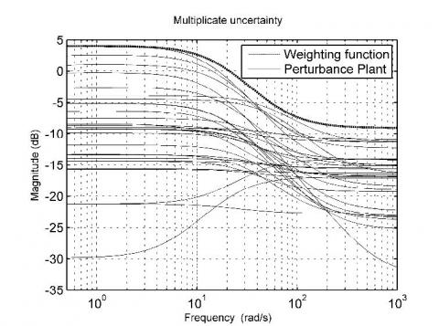
Figure 13 illustrates the set of ${{l}_{m}}$ frequency responses with 30 random uncertainties. It can be seen that the weighting functions ${{W}_{m}}$ bound all the possible perturbed models $G_p$ in the set ($∏$). According to the condition in Eq. (22), this result shows that the weighting requirement is well satisfied under given parametric uncertainty.
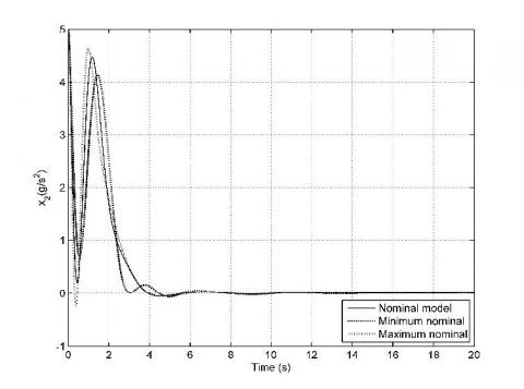
Figure 14 shows the time-domain performances of the closed-loop systems for boiling microchannel. Three dynamic models have been presented for the set of the perturbed systems: the minimum model with the minimum parameter value, the nominal model with average parameters, and the maximum model with maximum parameters. It is noted that the mass flowrate reaches the reference target in 6s with small overshoot. In comparison with some controllers such as active control of pressure drops using the feedback control [8] and flow control with electric field [12], the proposed controller offers better performance and robustness than those approaches under various uncertainties. In reality, other approaches do not directly include any uncertainty in the dynamical models.
Figure 13. Bode plots of uncertainty weighting function
Figure 14. Transient responses for the mass flowrate with robust controller
Besides the system response to the reference input, the disturbance input should be also attenuated by the active controller. In fact, the exogenous disturbances can impose additional heat to be dissipated from microchannel and require more control actions for these unanticipated demands. As shown in Figure 16, the disturbance with a magnitude of 1 g/s has been applied in addition to reference inputs for considering more practical cases. As illustrated, the effects of external disturbances are effectively eliminated by active controller. In case of constant magnitude, disturbances will be completely rejected in the microchannel system. Therefore, the boiling microchannel is stable under large disturbances, and the overall energy consumption can be minimized during plant operations. In practical, the external disturbances are often low-frequency signals, whereas sensor noises are high-frequency signals. Hence, it is necessary to eliminate the influence of noises on the boiling microchannel system. In Figure 17, the sensor noises with average magnitude of 7 units have been applied to the boiling microchannel system. It can be observed that 95% of noises have been eliminated. From the test results, the closed-loop system with active controller illustrated is insusceptible to external disturbances as well as sensor noises. It can be concluded that the proposed controller can offers not only robust stability but also robust performance against all uncertainties.
Figure 15. Transient responses for the rate of mass flowrate with robust controller
Figure 16. Time-domain system responses due to disturbance sensitivity with robust controller
Figure 17. Time-domain responses due to noise sensitivity with robust controller
This paper is focused on the dynamical analysis and robust control synthesis for boiling instability of microchannel system. For the nonlinear dynamical analysis, the phase portrait diagrams have been provided for the qualitative information of boiling microchannel. In addition, the bifurcation diagram is given for exploring dynamical behaviors of flow boiling when changing specific control parameters. The limit cycles and the periods of the pressure-drop oscillations are observed in two-phase flow boiling. Next, the linear model around the equilibrium point has been obtained for robust control synthesis. In general, flow boiling involves a highly complex dynamical phenomenon. Moreover, the parameter uncertainty, disturbance and sensor noise make it extremely difficult to control the microchannel system. The robust controller has been successfully applied to cope with these difficulties for guaranteeing optimal performance and ensuring also stabe plant operation. The time domain responses are provided by measuring rise time, peak time, maximum overshoot and settling time, especially, with ensuring the rise time of less than 2s for transient response. The simulation results show that the robust controller can cope with parametric variations and completely attenuate external disturbances and sensor noises in the steady-state, guaranteeing boiling stability. In addition, robust control system can deal with boiling flow instabilities leading to thermal and mechanical loadings and can maximize plant operation efficiency under various uncertainties. Consequently, the findings of this research will provide outstanding foundation on flow instability control and monitoring for plant operations.
Nguyen Ngoc Nam, Sang-Do Lee, Sam-Sang You, and Bui Duc Hong Phuc, both authors contributed equally to this work.
$A ̃$ cross-sectional area, ${{\text{m}}^{2}}$
(A,B,C,D) linearized state-space system matrix
$G(s)$ linear transfer function
$J$ lumped channel inertia, m
$k$ polytropic index
$K(s)$ linear controller
$L$ channel length,m
$\dot{m}$ mass flow rate , ${kg}.s^{-1}$
$P ̃$ pressure, Pa
$P(s)$ generalized plant
S sensitivity function
s Laplace variable
t physical time, s
V volume, m3
W weighting function
Greek symbols
$\rho $ density, ${kg}.s^{-1}$
$\Delta $ uncertainty
$ΔP ̃$ pressure drop,Pa
$\lambda $ eigenvalue
$\omega $ angular frequency, $\text{rad}\text{.}{{\text{s}}^{-1}}$
[1] Kandlikar SG. (2007). High flux heat removal with microchannels – a roadmap of challenges and opportunities. Heat Transfer Engineering 26(8): 5-14. https://doi.org/10.1080/01457630591003655
[2] Lee J, Mudawar I. (2009). Low temperature two phase microchannel cooling for high heat flux thermal management of defense electronics. IEEE Trans. Compo. Packag. Technol. 32(2): 453-465. https://doi.org/10.1109/TCAPT.2008.2005783
[3] Kandlikar SG, Bapat AV. (2007). Evaluation of jet impingement, spray and microchannel chip cooling options for high heat flux remove. Heat Transfer Engineering 28(11): 911-923. https://doi.org/10.1080/01457630701421703
[4] Thome JR. (2006). State of the art overview of boiling and two-phase flows in microchannels. Heat Transfer Engineering 27(9): 4-19. https://doi.org/10.1080/01457630600845481
[5] Garimella SV, Fleicher AS, Murthy JY, Keshavazi A, Prasher R. (2008). Thermal challenges in next generation electronic system. IEEE Trans Compo. Packagng Tech. 31(4): 801-815. https://doi.org/10.1109/TCAPT.2008.2001197
[6] Kakac S, Bon B. (2008). A review of two-phase flow dynamic instabilities in tube boiling system. International Journal of Heat and Mass Transfer 51(3-4): 399-433. https://doi.org/10.1016/j.ijheatmasstransfer.2007.09.026
[7] Kosar A, Kuo CJ, Peles Y. (2006). Suppression of boiling flow oscillation in parallel microchannel by inlet restrictor. ASME Journal of Heat Transfer 128(3): 251-260. https://doi.org/10.1115/1.2150837
[8] Zhang TJ, Peles Y, Wen JT, Tong T, Chang JY, Prasher R. (2010). Analysis and active control of pressure drop flow instabilities in boiling micro channel systems. International Journal of Heat and Mass Transfer 53(11-12): 2347-2360. https://doi.org/10.1016/j.ijheatmasstransfer.2010.02.005
[9] Zhang TJ, Wen TJ, Julius A, Peles Y, Jensen MK. (2011). Stability analysis and maldistribution control of two phase flow in parallel evaporating channels. International Journal of Heat and Mass Transfer 54(25-26): 5298-5305. https://doi.org/10.1016/j.ijheatmasstransfer.2011.08.013
[10] Doyle J. (1982). Analysis of feedback system with structure uncertainty. IEE Proceeding D - Control theory and Applications 129: 242-250. https://doi.org/10.1049/ip-d.1982.0053
[11] Skogestad S, Postlethwaite I. (2005). Multivariable feedback control analysis and design. 2nd Edition, John Wiley & Sons Ltd, England.
[12] Lackowski M, Krupa A, Butrymowicz D. (2013). Dielectrophoresis flow control in microchannel. Journal of Electrostatics 71(71): 912-925. https://doi.org/10.1016/j.elstat.2013.07.004