Abed Meghdir* | Tawfik Benabdallah | Ahmed Z.E. Dellil
© 2019 IIETA. This article is published by IIETA and is licensed under the CC BY 4.0 license (http://creativecommons.org/licenses/by/4.0/).
OPEN ACCESS
In this paper we have numerically treated the thermal and dynamic aspect of different prismatic bodies simulating electronic components, heated and mounted on the lower wall of a channel. These components are cooled by forced convection using a turbulent flow flowing along the channel and an impinging jet flowing from the upper wall perpendicularly to them. The fluid used is air of which we vary the Reynolds number in order to see its impact on the component cooling. We opted for four different geometries of the prismatic body taken in the same working conditions. We compared the results obtained to propose one of the geometries which will permit a better evacuation of the heat, thus a good cooling of the component.
By combining an unstructured mesh with the finite volume method, the solution is obtained by using the SIMPLE algorithm (pressure-velocity coupling). Turbulence is modeled using the so-called Shear Stress Transport (SST) model to evaluate the heat exchange in these configurations. This numerical study is carried out with the code ANSYS.CFX 14 to evaluate the thermal exchanges.
cooling of electronic components, SST turbulence Model, heat transfer, forced convection
Forced convection air cooling of electronic components is of great importance as it ensures their correct functioning. It avoids any malfunction, causing a risk of loss of the characteristics and performance of the electronic system caused by heat dissipation in these components.
As soon as an electronic component is crossed by an electric current, it tends to produce heat (loss by Joule effect). This heat is not perceptible for components with low current flow, but it is significantly more important for components where a high electric current is circulating. So we must evacuate all the heat produced by the component immediately after its production. If the heat dissipation is less than its production, the electronic system is increasingly heated and can lead to the malfunction or even irreversible damage to the component. We must therefore ensure that the system does not exceed a given temperature allowed by the manufacturer.
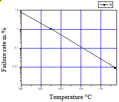
Figure 1 shows that a small increase of the operating temperature causes an exponential increase in the number of failures Hamouche [1].
The thermal effects can manifest in different ways: By a temperature drift of the components, causing significant variations in electrical performance. Or by a rupture of the welds connecting the component to the substrate, thus causing a partial or total failure. The cooling phenomenon of electronic components has been the subject of many scientific works.
The cooling phenomenon of electronic components has been the subject of many scientific works. Among the first precursors, Castro & Robins in their experimental study they measured the velocity field around a cube mounted on a plate [2]. They found that in the recirculation zone at the rear of the cube, the wake zone and the size of the vortex depended on boundary conditions at the entrance.
Figure 1. Variation of the failure rate
Larousse, Martinuzzi and Tropea, studied experimentally studied the flow field around prismatic obstacles of different dimensions mounted on a surface [3-5]. The main characteristics of the flow have been highlighted such as: the horseshoe vortex on the front of the cube, the vortex in the wake of the obstacle, the flow recirculation on top, and on the lateral sides. They also found that the horseshoe vortex was unstable, non-periodic, and the vortex disintegrates in the wake of the cubic obstacle.
Sakakibara et al. [6], have experimentally studied the swirling structure effect and the heat transfer in the stagnation region of an impinging jet. For various values of the jet Reynolds number (2000 <Re<20,000), they found the existence of a pair of counter-rotating vortices in the stagnation zone, which by amplifying favors the heat transfer in this zone.
Meinders [7], by taking Reynolds numbers between 2750 <ReH <4970, they experimentally studied the local convective heat transfer of a cube placed in a turbulent flow in a channel. The distribution of the local heat transfer coefficient was obtained from the surface heat flux, which was evaluated from the inlet temperature. The temperature of the epoxy layer and the temperature distribution of the cube surface, were acquired by infrared thermography. Meinders also studied, the flow field using a laser Doppler anemometer, and flow visualizations aiming to correlate the local heat transfer with the flow model. He concluded that the complex vortex structure around the cube particularly on the top and side faces provoked a large variation in the local convective heat transfer.
Rundstrom et al. [8], used two different turbulence models, a model (ν2 -f) and a Reynolds constraint model (Route Mean Square RSM) with a two-layer model in the region close to the wall. These models were used to analyze the flow around a cube placed at the center of a plate at the base of a pipe, which is subjected to both an axial transverse flow and an impinging jet perpendicular to the upper face of the cube. The main difference is that the SST model produces a higher turbulent kinetic energy (K) level in all regions, and the largest differences are in the stagnation region at the top of the cube.
Tummers wrote an article on the flow structure and surface temperature distribution of a heated cube, mounted on a wall of a channel and subjected to cooling by the combined action of the channel flow and an incident jet from a constant diameter orifice [9]. The local flow structure in terms of flux separation and reattachment and the winding separating the shear layers, has an influence on the local temperature distribution at the surface of the cube.
Bazylak et al. have made an estimated numerical analysis of the heat transfer due to a set of sources arranged on the bottom wall of a horizontal enclosure [10]. They found that optimal heat transfer rates and the onset of thermal instability depend on the length and spacing of the sources and the aspect ratio of the enclosure. The transition from conductive to convective regime is characterized by a range of Rayleigh number values; and decreases by increasing the length of the source. For small lengths of the source, the structure of the Rayleigh-Benard cell is transformed into small large cells, which means that we are in the presence of an important heat transfer and a bifurcation characterized by the existence of instabilities in the physical system was obtained.
Alexander Yakhot et al. [11], used an immersed-boundary method to perform a direct numerical simulation (DNS) of flow around a wall-mounted cube in a fully developed turbulent channel for a Reynolds number Re=5610, based on the bulk velocity and the channel height. Instantaneous results of the DNS of a plain channel flow were used as a fully developed inflow condition for the main channel. The results confirm the unsteadiness of the considered flow caused by the unstable interaction of a horseshoe vortex formed in front of the cube and on both its sides with an arch-type vortex behind the cube. The time-averaged data of the turbulence mean-square intensities, Reynolds shear stresses, kinetic energy and dissipation rate are presented. The negative turbulence production is predicted in the region in front of the cube where the main horseshoe vortex originates.
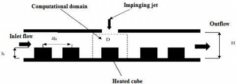
Rundstrom and Moshfegh conducted numerical simulations in mixed convection to predict the main turbulence characteristics for a jet flow on the heated wall of a cube (Figure 2) [12]. Two different simulations were carried out and compared to the experimental results; that of the Large Scale Simulations (LSS) and the Reynolds Tension Model (RTM). The results revealed that the structure of the flow is very complex. There are several flows related to phenomena, such as points of stagnation, separations and re-circulations. The results show that the temperature simulation by (LSS) is in better agreement with the experimental results relative to the simulation (RTM), particularly in the stagnation zone. In addition, the prediction of temperature-length scales by (LSS) is close to the experimental measurements on the front and rear faces of the cube compared to (RTM) prediction.
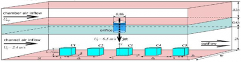
Popovac & Hanjalic have studied numerically at a large-scale (LES) [13], the cooling of an electronic component. The configuration consists of a row of five cubes mounted on the flat channel wall with a perpendicular jet pointed above the heated cube, its axis aligned with the cube’s front wall (Figure 3). After several tests of change in the position of the jet axis, results have shown that the complex interaction of the two jets with the cube produced several vortex structures around the cube governing the local heat transfer on the cube’s surfaces.
Figure 2. Schematic representation of the experimental installation [10]
Figure 3. Schematic representation of the experimental Installation [11]
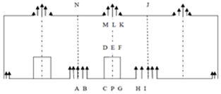
Bhoite and Narasimham simulated mixed turbulent convection in a shallow cavity (with and without partitions) containing a series of blocks (Figure 4) [14]. A series of Reynolds and Grashof numbers were taken into account in the calculations. The results show that the increase in Reynolds numbers tends to create an increasing force circulation region in the base zone; in addition, the buoyancy effect becomes insignificant beyond a certain Reynolds number (Re=5×10⁵). The maximum adimensional temperatures that were obtained are almost the same, whether for partitioned or unpartitioned geometry.
Figure 4. Physical model containing a heat source [14]
Ratnam and Vengadesan simulated the characteristics of vortex structures and the heat transfer coefficient associated with a cubic obstacle mounted on the lower wall of a channel (Figure 5) [15]. The calculations were performed using five turbulence models. The results showed that the improved (K-ω) model, has better agreement with direct numerical simulation (DNS), as well as experimental study and non linear models (K-ε) gave better predictions than models standard (K-ε) and (K-ε) with a low Reynolds number. The maximum and minimum heat transfer coefficients are respectively close to the points of attachment and the circulation zone.
Figure 5. The computational domain of the study [15]
Yukun Dai [16] studied the effect of the interval between two wall-mounted square cylinders was conducted. After the comparison of force coefficients, pressure and velocity field, the strongest interaction between the two cylinders was in the case 1 with L=h, where unique reattachment and cavity flow were found inside the interval. However, with the increasing interval, the reattachment and the cavity flow disappear and the two cylinders become independent in the cases with L=2h and L=5 h. The weakest interaction was found for the case 3 with L=5 h, in which the resulting drag coefficient CD showed less than 5% and the lift coefficient showed less than 8 % difference relative to the one cylinder simulation. The formations of each vortex, low pressure and low velocity zone have been explained.
Figure 6. Definition of the computational domain
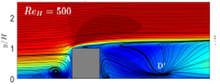
Carlos Diaz-Daniel et al. [17] A wall-attached cube immersed in a zero pressure gradient boundary layer is studied with the Direct Numerical Simulations (DNS) at various Reynolds numbers ReH (based on the cube height and the free-stream velocity) ranging from 500 to 3 000 (Figure 7).
The cube is either immersed in a laminar boundary layer (LBL) or in a turbulent boundary layer (TBL), with the aim to understand the mechanisms of the unsteady flow structures generated downstream of the wall-attached cube. The mean locations of the stagnation and recirculation points around the cube immersed in a TBL are in good agreement with reference experimental and numerical data; even if in those studies the cube was immersed in a turbulent channel. In the TBL simulation, a vortex shedding can be identified in the energy spectra downstream of the cube, with Strouhal number of St=0:14. However, the frequency of the vortex shedding is different in the LBL simulations, showing a significant dependence on the Reynolds number. Furthermore, in the TBL simulation, a low frequency peak with St= 0:05 can be observed far away from the boundary layer, at long streamwise distances from the cube. This peak cannot be identified in the LBL simulations nor in the baseline TBL simulation without the wall-attached cube.
Figure 7. Mean flow streamlines and time-averaged streamwise velocity contours at ReH=500
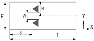
Sahin et al. [18], studied, the effects of equilateral triangular bodies placed in the channel on heat transfer and pressure drop characteristics were examined numerically. Reynolds number varied from 5000 to 10000. The effects of the blockage ratio at constant edge length (B=20 mm) and Reynolds number of triangular bodies were investigated. An RNG based k-ε method was used and a constant surface temperature was applied to the bottom wall. The numerical results were presented with respect to temperature contours, local and mean Nusselt number, local and mean surface friction factor changes and heat transfer enhancement ratios. The results showed that the presence of the equilateral obstacles in the flow field enhanced the heat transfer. Temperature distributions behind the bodies were affected by the position of the triangles and the Reynolds number and changed greatly in the vertical direction along the x distance beyond the bluff bodies. The intensity of the oscillations decreased with the increase of the Reynolds number. It was observed that for all cases overall heat transfer enhancement was provided. It was found that the highest values of OHTE were reached at W/B=0 and Re=5.0 and lowest were at W/B=1 and Re=10.0
Figure 8. Computational domain
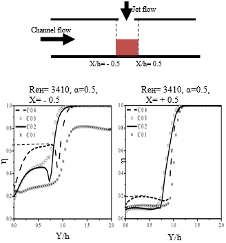
Masip et al. [19], experimentally studied the influence of the Reynolds numbers of the impinging jet (Rej) and that of the channel air flow (ReH), on the flow structure. Three Reynolds numbers of the channel fllow were used (3410, 5752, 8880), while taking the ratio Rej/ReH equal to 0.5, 1.0, 1.5 respectively.
The results showed that the impinging jet does not reach the upper wall of the cube in the event of a low Reynolds number, eliminating the existence of the horseshoe vortex on the top wall and changing the characteristics of the wall flow in the region above the cube.
Nemdili et al. [20], studied numerically the case of a heated cube, simultaneously exposed to a transverse flow and a perpendicular jet, they varied the value of the Reynolds number and modified the shape of the cube by chamfering the upper edge. Their study covered the quantification of the thermal contribution related to this geometric change and concluded that the overall heat flux exchanged through the cube is increased about 26% of its base value for the case where Rej/ReH=1.5 and a chamfer value s=4mm.
Villalba et al. [21], used Large Eddy Simulation to investigate a forced convection heat transfer in the flow around a surface mounted cylinder with, height to diameter ratio of 2.5, a Reynolds number based on the cylinder diameter of 44000 and Prandtl number of 1. The surface of cylinder is heated while the bottom wall and the inflow are kept at a lower fixed temperature. The boundary layer had a thickness of about 10% of the cylinder height. As result, the heat transfer coefficient is strongly affected by the free end of cylinder, the flow over the top being downwashed behind the cylinder and a vortex-shedding process does not occur in the upper part, leading to a lower value of the local heat transfer coefficient in that region. In the lower region, vortex-shedding takes place leading to higher values of the local heat transfer coefficient.
Curley and Uddin [22], have studied numerically using the Direct Numerical Simulation (DNS) a surface mounted cube in a channel flow with a Reynolds number of 5610 based on the cube height. The velocity was simulated using the fifth order compressible finite difference code. The results of the simulations obtained were compared and validate with the numerical and experimental results of other works already published. Their study leads recommendations on input parameters, boundary conditions and the simulation domain to prepare a DNS more conform to the experimental results. They highlighted a system of six horseshoe vortices upstream of the cube, two counter-rotating vortices along the sides of the cube, and an arch-shaped vortex downstream of the cube.
Hearst et al. [23]. They studied experimentally the influence of turbulence on the flow around a wall mounted cube in a turbulent boundary layer using particle image velocimetry and hot wire anemometry. They used a free stream turbulence to generate turbulence boundary layer profiles with at the cube height, the normalized shear is fixed and turbulence intensity is adjustable. The Reynolds number of boundary layer Rex=18.105 and the ratio of cube height to boundary layer thickness h/δ=0.47. They have found that for the conditions investigated, the stagnation point on upstream side and the reattachment length in of the cube are independent of incoming profile. They also deduce that the wake length decreases for increasing intensity. They conclude that the wake shortening is a result of heightened turbulence levels promoting wake recovery from high local velocities and the reduction in strength of a dominant shedding frequency.
Masip et al. [24], experimentally studied the influence of the Reynolds numbers of the impinging jet (Rej) and that of the channel air flow (ReH), on the flow structure. Three Reynolds numbers of the channel flow were used (3410, 5752, 8880), while taking the ratio Rej/ReH equal to 0.5, 1.0, 1.5, respectively. The results showed that the impinging jet does not reach the upper wall of the cube in the case of a low Reynolds number, eliminating the existence of the horseshoe vortex on the top wall and changing the characteristics of the wall flow in the region above the cube.
Heidarzadeh et al. [25], studied numerically a turbulent fluid flow and convective heat transfer over the wall mounted cube in different flow angle of attack using large eddy simulation. Dynamic Smagorinsky subgrid scale model were used in this study. Angles were in the range 0≤θ≤45° and Reynolds number based on the cube height and free stream velocity was 4200. The numerical simulation results were compared with the experimental data of Nakamura et al. Characteristics of fluid flow field and heat transfer compared for four angles of attack. Flow around the cube was classified to four regimes. They found that the local convective heat transfer from the faces of the cube and plate are directly related to the complex phenomena such as horse shoe vortex, arch vortexes in behind the cube, separation and reattachment. Results show that overall convective heat transfer of cube and mean drag coefficient have maximum and minimum value at θ = 0 and θ = 25°, respectively.
Sercan Dogan et al. [26], have employed turbulence models to investigate the flow characteristics around a surface-mounted cube (Figure 9) at Re = 3700 based on the edge length of the cube in terms of Computational Fluid Dynamics (CFD) and then compared with experimental results in the literature. Normalized and time-averaged results of velocity vector fields, streamwise and cross-stream velocity components, vorticity contours and streamline patterns have been numerically obtained by using k-ε Re-Normalization Group (RNG), k-ω Shear Stress Transport (SST) and Large Eddy Simulation (LES) turbulence models. They also found that “LES” turbulence model has presented the best prediction of hydrodynamic characteristics for the body.
Our study focuses on the search for a way to improve the heat transfer from the component to the air flow, because the energy dissipated in the heating resistance of a component is not carried away in its totality by the air flow. For this purpose the objective is to show the impact of the geometry of the component in the presence of the velocity variations of the channel flow and the impinging air jet on the component cooling.
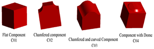
We have opted for four different geometrical configurations as shown in the Figure 10.
Figure 9. Flow domain on the XY plane
Figure 10. The four proposed geometries
1.1 Turbulence Model SST (Shear Stress Transport)
For solving the problem of cooling the components, we used the model of Shear Stress Tensor (SST) introduced in 1994 by Menter [27]. The formulation of the SST model is based on physical experiments and attempts to predict solutions to typical engineering problems. It demonstrated these possibilities of accurate predictions of separation in numerous cases. Under an unfavorable pressure gradient, the detachment plays an important role near the wall (intensification of heat transfer). It activates the Wilcox [28] model (K-ω) in the area near the wall and the Launder and Spalding [29] model k-ε for the rest of the flow.
The idea behind the SST model is to combine the models k-ε and K-ω using depreciation coefficient f1 , f1 is equal to 1 near the wall and zero away from the wall. The execution of the Wilcox model can be used without potential errors and the formulation of the SST model is as follows:
$\frac{\partial (pk)}{\partial t}+\frac{\partial (\rho {{U}_{j}}k)}{\partial {{x}_{i}}}={{P}_{k}}-{{\beta }^{*}}\rho k\omega +\frac{\partial }{\partial {{x}_{i}}}({{\Gamma }_{k}}\frac{\partial k}{\partial {{x}_{i}}})$ (1)
$\frac{\partial (p\omega )}{\partial t}+\frac{\partial (\rho {{U}_{j}}\omega )}{\partial {{x}_{j}}}=\frac{\gamma }{{{v}_{t}}}{{P}_{k}}-\beta \rho {{\omega }^{2}}+\frac{\partial }{\partial {{x}_{j}}}({{\Gamma }_{\omega }}\frac{\partial \omega }{\partial })+\rho {{\sigma }_{\omega 2}}\frac{1}{\omega }\frac{\partial k}{\partial {{x}_{j}}}\frac{\partial \omega }{\partial {{x}_{j}}}$ (2)
The variable definition:
Pk represents production of turbulent kinetic energy due to the gradient of the average velocity:
${{P}_{k}}={{\tau }_{ij}}\frac{\partial {{U}_{i}}}{\partial {{x}_{j}}}$ (3)
${{\tau }_{ij}}={{\mu }_{t}}(2Sij-\frac{2}{3}\frac{\partial {{U}_{k}}}{\partial {{x}_{k}}}{{\delta }_{ij}})-\frac{2}{3}k{{\delta }_{ij}}$ (4)
${{S}_{ij}}=\frac{1}{2\left( \frac{\partial {{U}_{i}}}{\partial {{x}_{j}}}+\frac{\partial {{U}_{j}}}{\partial {{x}_{i}}} \right)}$ (5)
${{\mu }_{t}}=\frac{\rho {{a}_{1}}k}{\max ({{a}_{1}}\omega ,\Omega {{F}_{2}})}$ (6)
$\phi \text{=}{{F}_{1}}{{\phi }_{1}}+(1-{{F}_{1}}){{\phi }_{2}}$ (7)
$F_1=tanh(arg_1^4 )$ (8)
$\arg \_1=\min [\max ((\frac{\sqrt{k}}{\beta *\omega d'}),(\frac{500v}{{{d}_{2}}\omega }),\frac{4\rho \sigma \omega 2k}{C{{D}_{k\omega }}^{{{d}^{_{2}}}}})]$ (9)
$C{{D}_{k\omega }}=\max [2\rho {{\sigma }_{{{\omega }^{2}}}}\frac{1}{\omega }\frac{\partial k}{\partial {{x}_{i}}}\frac{\partial \omega }{\partial {{x}_{i}}},{{10}^{-20}}]$ (10)
$F_2=tanh(arg_2^2)$ (11)
$\arg \_2=\max (\frac{2\sqrt{k}}{\beta *\omega d},\frac{500v}{{{d}_{2}}\omega })$ (12)
The constants definition are:
The constants of the model K-ω are: $σ_k1=0.85$,$σ_ω1=0.65$,$β_1=0.075$
The constants of the model k-ε are: $σ_k2=1.00$,$σ_ω2=0.856$,$β_2=0.0828$
The SST constants are: $β^*=0.09$,$ α_1=0.31$
In order to evaluate the thermal exchanges in these configurations of electronic components, numerical simulations were conducted with the CFX 14 code.
To simulate flows through the most complex geometries, this software is divided into important modules: The ICEM CFX.CFD: allows the preparation of the geometrical configuration and the generation of two types of meshes, the TETRAHEDRAL and HEXAHEDRAL mesh. The CFX-Pre prepares the initial and boundary conditions, and solves the equations using models available. The CFX-Post displays the different results on the screen.
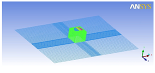
Figure 11. Representation of the computational domain
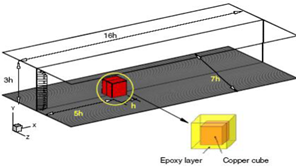
The Figure 11 represents our computational domain, composed of a rectangular channel in which the electronic component is placed on its lower wall. The electronic component heated to 75°C is cooled by two air flows at 20°C, one of which flows longitudinally and the other in the form of an impinging jet perpendicular to the upper surface of the component. In our simulations we vary the Reynolds number of the channel flow, ReH = 3410, 5752, 8880 and α so as to be in accordance with the experimental study.
With regard to the impinging jet, the Reynolds numbers ReJ are calculated from a coefficient α such that
- α=ReJ / ReH=0.5 (channel flow is twice that of the jet).
- α=ReJ / ReH=1 (channel flow is equal to that of the jet).
- α=ReJ / ReH=1.5 (jet flow is greater than that of the channel flow).
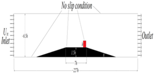
2.1 Boundary conditions
At the inlet of the channel we have imposed a velocity for the main flow which is calculated from the Reynolds number ReH and another velocity for the secondary flow corresponding to that of the jet and calculated from α =ReJ/ReH. At the outlet of the channel, a zero pressure gradient was taken. The two top and bottom walls are considered to be adiabatic and the side walls as symmetrical. The simulation is reproduced for the four different geometric configurations. The aim is to verify if the geometry, the variation of the Reynolds number of the air flow of the channel (ReH) and the coefficient α affect the cooling efficiency.
To validate our digital work, we tested three different meshes (Table 1), and finally selected only the mesh comprising 552888 elements and 532720 nodes for each case studied as being the optimal mesh.
Table 1. Tested meshes
|
|
Type |
elements |
nodes |
|
Grid 1 |
hexahedral |
5 52888 |
5 32720 |
|
Grid 2 |
hexahedral |
887447 |
851280 |
|
Grid 3 |
hexahedral |
1264327 |
1237289 |
Figure 12. Representation of the computational domain
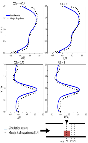
We validated our simulations results with the experimental work of Massip et al. [24], who validated his results with those of Meinders [30]. The velocity profiles obtained numerically using the SST model for four different positions as shown in Figure 12.
Figure 12. Longitudinal velocity profile at Z/h=0 for ReH=3410 and α =0.5
3.1 Thermal profile
3.1.1 Reynolds number ReH constant and α variable
In addition to the effects of the Reynolds number of the channel air flow ReH and the ratio α, we wanted to highlight the impact of the component’s geometry on its cooling.
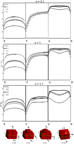
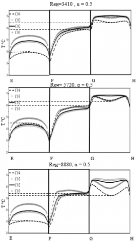
Figure 13, shows the temperature variation along the EFGH line at the intersection of the component with the horizontal plane XZ at Y/h=0.5. Reynolds number ReH = 3410 is kept constant and α=0.5, 1 and 1.5.
* For α = 0.5, we note that the curves are respectively similar according to the three segments EF, FG, GH for the four components.
It should be noted that; according to EF this is where the temperature is the lowest compared to FG and GH, because the front face of the component is directly exposed to the air flow of the channel. Moreover, the component C04 is the one that is best cooled according to the three lines EF, FG, GH compared to the other three components.
* For α=1, there is a slight improvement in cooling along the lateral and rear faces of the components compared to case α = 0.5.
* For α = 1.5; there is a clear improvement in the cooling of the side and rear faces, especially for the component C04. This is due to the increase in the air flow of the impinging jet which is greater than that of the channel.
It should be said that for ReH=3410, if we increase the ratio α, we improve the cooling of the components according to all their faces (front, rear and lateral). The component C04 is the most cooled.
Figure 13. Temperature profiles comparison along line EFGH at Y/h=0.5 for ReH =3410 and α = 0.5, 1, 1.5 for the four different geometries
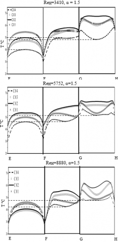
3.1.2 Reynolds number ReH is variable and α is constant
Figure 14. Temperature profiles comparison along line EFGH at Y/h=0.5 for ReH =3410, 5752, 8880 and α=0.5
In this section, we wanted to see the effect of change in the channel air flow (ReH) over the cooling of the four components. For this purpose we have varied the Reynolds number ReH and kept the value of α constant (see Figure 14).
Figure 14 shows fairly well that by increasing the channel air flow (ReH) and maintaining α’s ratio constant at 0.5, we can cool the components in their globality. For ReH =8880, there is a clear improvement in the cooling of the component C04 according to its different faces (front, lateral and rear), compared to the cases where ReH=3410 and 5752.
In Figure 15, we varied the channel air flow and increased the air flow of the impinging the jet so that α = 1.5.
By increasing both air flows (ie α = 1.5 and ReH = 3410, 5752 and 8880), it is possible to cool the components even more on all faces. Due to the fact of increasing the values of α and ReH, the flow is deflected towards the rear and the laterals faces of the components. Under these same conditions, the C04 component remains the one that best meets our requirements.
Figure 15. Temperature profiles comparison along the line EFGH at Y/h=0.5 For ReH =3410, 5752, 8880 and α=1.5 for the four different geometries
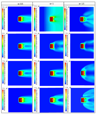
3.2 Contours of temperatures according to the plane XZ with Y/h= 0.5
3.2.1 Reynolds number ReH is constant and α is variable
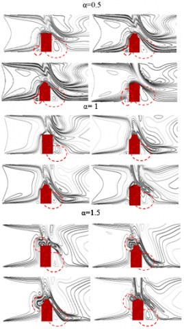
Figure 16 represents the temperature contours along a plane XZ situated at a height Y/h= 0.5, for different values of α and ReH constant.
In the case of α = 0.5, it is observed that the flow of the channel carries almost all the heat at the rear of the components. When α =1, there is a shared diffusion between the flow of the channel and that of the impinging jet. For α = 1.5, there is a presence of turbulence all around the component giving rise to a clear cooling compared to the other two cases.
The component C04 presents a better cooling because this geometry favors the presence of several vortices around the component when α takes the values 1 and 1.5.
Figure 16. Temperature contours comparison according
the plane XZ at Y/h=0.5 for ReH =3410 and α=0.5,1,1.5
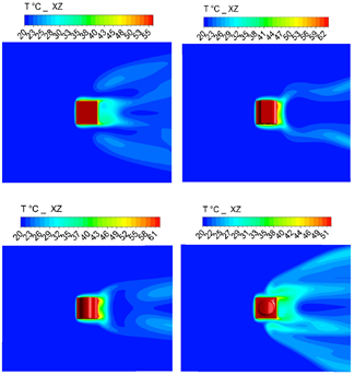
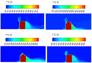
3.2.2 Reynolds number Re H =8880 and α =1.5
In Figures 17a, we represent the temperature contours along the XZ plane at a height Y/h= 0.5 for ReH = 8880 with α = 1.5 and in figures 17b, along the XY plane at Z/h= 0.
By increasing the channel air flow (ie ReH = 8880) with a larger impinging jet (ie α = 1.5), we observed that from the temperature scales, the components are more cooled compared to the case where ReH = 3410. We also see a significant diffusion of heat towards the rear of component, evidence of good heat transfer for element C04. The component C04 is the one that undergoes a net lowering of the temperature, thus an improvement of its cooling compared to the previous case.
Figure 17a. Temperature contours comparison along
the plane XZ à Y/h=0.5 for ReH =8880 and α =1.5
Figure 17b. Temperature contours comparison according the plane XY à Z/h=0 for ReH =8880 and α =1.5
3.3 Determination of cooling efficiency
Afterwards we wanted to determine the efficiency of the cooling following two vertical lines on the front and rear faces of the components as shown in figure 18.a and b. The efficiency is calculated from the following equation:
$η=\frac{T_{component}-T_{ref}}{T_{component}-T_{in}}$ (13)
where
Tcomponent is the temperature of the component.
Tref is the flow temperature at the position X/h.
Tin is the air inlet temperature.
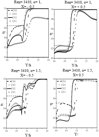
Figure 18a. Comparison of cooling efficiencies for ReH=3410 and α=0.5, 1, 1.5 following the vertical lines at X/h=-0.5 and 0.5 for Z/h=0
Figure 18a clearly shows that the front face of the components has the best cooling efficiency for the various components. Around the middle of the component C04 the efficiency reaches up to 65%. Regarding the rear face, it can be seen that the efficiency increases when α increases. Following the line X / h = 0.5; for the component C04, the cooling efficiency goes from 15 to 20 % for α=0.5 to from 30 to 50 % for α=1.5. Whereas for the simple cubic element C01 it varies between 10 to 15% for α=0.5, and from 18 to nearly 25 % for α=1.5.
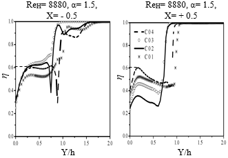
For Figure 18.b, we increased the value of the Reynolds number to Re H=8880 and took α=1.5.
Figure 18b. Comparison of cooling efficiencies for ReH=8880 and α=1.5, along the vertical lines at
X/h=-0.5 and 0.5 for Z/h=0
We noticed that the front face still remains the most cooled face, because it is directly exposed to the flow of the channel. However, in this case the rear face is even cooler compared to the previous cases in Figure 13.a. Its efficiency now varies between 40 to 60 % for the C04 component, whereas for the simple cubic element C01 it varies between 35 to 50 %
In the same way we wanted to see the evolution of the efficiency along the horizontal lines EF and GH located respectively on the front and rear of the components at a height of Y/h=0.5 (see Figure 19).
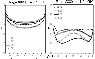
Figure 19. Comparison of cooling efficiencies for ReH=8880 and α=1.5, following the horizontal lines EF and GH at Y/h=0.5
In figure.19, the component C04 which is best cooled, has a cooling efficiency that varies from 80 % at the extremities of the line EF, to 60 % in the middle of the line. At the rear face of the component, along the line GH, the efficiency goes from 60 % at the extremities G and H, to 50 % in the middle of the line. We noticed that when α goes from 0.5 to 1 the efficiency increases a little, while for α=1.5, the increase is important along GH.
3.4 Dynamic profile
After studying the thermal aspect, we are interested in the dynamic profile to argue the thermal profiles obtained previously.
Figures 20.a and b represent the velocity contours along the XY plane at Z/h=0, for ReH=3410 and α=0.5, 1, 1.5 and for ReH=8880 and α=1.5, respectively.
Figure 20a. Comparison of velocity contours along the plane XY at Z/h=0 pour ReH =3410 and α=0.5, 1, 1.5
Figure 20b. Comparison of velocity contours along the plane XY at Z/h=0 pour ReH =8880 and α=1.5
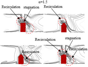
On Figures 20a and 20b, we can clearly see the effect of α (ratio of flow rates) on the velocity contour. When α=0.5, we notice that the impinging jet is deviated from the upper surface of the component, however, when α increases either to α=1 or 1.5, the jet is directed towards the upper face where a stagnation and the recirculation zones appears.
The detachment of the flow observed when we pass from the simple geometry to the three other geometries, causes the birth of these vortices. The heat flux exchange importance is influenced by these vortices.
The vortex, which develops around the jet, increases and takes different forms for the high values of ReH.
We also note the appearance of recirculation upstream and downstream of the component, witnessed the birth of two vortices. These vortices intensify with increased value of α and ReH as well as the changing shape of the component.
The present work is based on the finite volume method and deals with the cooling of electronic components, placed in a channel where air flows, and is subjected to an impinging jet. The SST model for the resolution of temperature and velocity profiles allows to accurately reproduce the flow. Several experimental and numerical works have treated this subject by varying the boundary conditions or solving methods (K-ε, K-ω, LES, DNS), while taking the same geometry of a simple cubic element.
Our work is to change the geometry of the component and to see its impact on cooling. For this purpose we opted for four different geometries (C01, C02, C03 and C04), taken under the same boundary conditions (ReH and α), as the experimental study of Massip et al. [16], then we compared the results.
We have shown that among the factors that influence the cooling efficiency, such as the different flow regimes (variation of the Reynolds number), the different flow ratios α; the geometry of the element was of a great importance, because it helps to improve the cooling efficiency.
We also found that among the four geometries, it is the fourth element C04 which gave us a better cooling and whose efficiency approaches 50% on its upstream, downstream and lateral faces, compared to the simple cubic element which is around 30%. This is due to the fact that this geometry favors turbulence, thus heat transfer.
We can conclude that the combined effect of the geometry with the channel air flow and the impacting jet, considerably favors the cooling of the components.
|
D |
Diameter of the jet equal to 12 mm |
|||
|
CP |
specific heat, J. kg-1. K-1 |
|||
|
f1 |
Dumping coefficient |
|||
|
K H |
Turbulent kinetic energy thermal Channel height equal to 30 mm |
|||
|
PK |
production of turbulent kinetic energy |
|||
|
h ReH Rej Sij T Tref Tcomponent Tin Ui,Uj |
Cube edge equal to 15 mm Reynolds number of channel airflow Reynolds of the impinging jet Mean strain rate tensor Temperature; characteristic time scale Flow temperature at the position X/h °C Temperature of the component °C Air inlet temperature °C Mean velocity in tensor notation |
|||
|
Greek symbols |
||||
|
a |
Ratio of Reynolds Rej/ReH |
|||
|
β* |
Coefficient of Thermal expansion |
|||
|
Γ |
Coefficient of diffusion |
|||
|
δij |
Kronecker symbol |
|||
|
ω |
Specific dissipation rate s-1 |
|||
|
ε |
Turbulence dissipation rate m2.s-3 |
|||
|
f |
Generalized variable |
|||
|
µ φ λ υ νt ρ τij η |
dynamic viscosity, kg. m-1.s-1 Density of the flux W. m-2 Thermal conductivity w / m.°c Kinematic viscosity kg / m.s Turbulent kinematic viscosity m2.s-1 density of the fluid kg / m3 Reynolds stress tensor Efficiency |
|||
|
Subscripts |
||||
|
H |
Channel |
|||
|
j |
impinging jet |
|||
|
ref component in |
Reference Component Inlet |
|||
[1] Hamouche A. (2012). Study of mixed convection in a channel containing sources of heat. PhD Thesis. University of Mentouri-Constantine, Constantine, Algeria.
[2] Castro IP, Robins AG. (1977). The flow around surface mounted cube in uniform and turbulent streams. Journal of Fluid Mechanics 34(7): 307-335. https://doi.org/10.1017/S0022112077000172
[3] Larousse A, Martinuzzi R, Tropea C. (1991). Flow around surface-mounted, three-dimensional obstacles. Eighth Symposium on Turbulent Shear Flows. TU, Munich/Germany 1: 1441-1446. http://dx.doi.org/10.1007/978-3-642-77674-8 10
[4] Martinuzzi RJ. (1993). Experimental untersuchun der umstroming wandgebundener, rechteckiger, prismatischer. Ph.D Thesis. Erlangen, Germany.
[5] Martinuzzi RJ, Tropea C. (1993). The flow around surface mounted, prismatic obstacles in a fully developed channel flow. J. Fluids Eng. 115: 85-92. http://dx.doi.org/10.1115/1.2910118
[6] Sakakibara J, Hishida K, Maeda M. (1997). Vortex structure and heat transfer in the stagnation region of an impinging plane (velocimetry image and laser induced fluorescence). Int. J. Heat and Mass Transfer 40: 3163-3176. http://dx.doi.org/10.16/S0017-9310(93)00367-5
[7] Meinders ER. (1998). Experimental study of heat transfer in turbulent flows over wall-mounted cubes. Ph.D. Thesis. Delft University of Technology, The Netherlands.
[8] Rundstrom D, Moshfegh B. (2007). Numerical investigation of flow behavior of an impinging jet in a cross-flow on a wall mounted cube using RSM and v2-f turbulence models. Progress in Computational Fluid Dynamics 7(6): 311-322. http://dx.doi.org/10.1504/PCFD.2007.014681
[9] Tummers MJ, Filkweert MA, Anjalic K, Rodink R, Moshfegh B. (2005). Impinging jet cooling of wall mounted cubes. Engineering Turbulence Modeling and Experiments 773-782. https://doi.org/10.1016/B978-008044544-1/50074-1
[10] Bazylak A, Djilali N, Sinton D. (2006). Natural convection in an enclosure with distributed heat sources. Numerical Heat Transfer, Part A 49: 655-667. http://dx.doi.org/10.1080/10407780500343798
[11] Yakhot A, Liu H, Nikitin N. (2006). Turbulent flow around a wall-mounted cube: A direct numerical simulation. International Journal of Heat and Fluid Flow 27: 994–1009. http://dx.doi.org/10.1016/j.ijheatfluidflow.2006.02.026
[12] Rundström D, Moshfegh B. (2008). Investigation of heat transfer and pressure drop of an impinging jet in a cross-flow for cooling of a heated cube. ASME J. Heat Transfer 130(12): 1-13. http://dx.doi.org/10.1115/1.2969266
[13] Popovac M, Hanjalic K. (2007). Large-eddy simulations of flow over a jet-impinged wall-mounted cube in a cross-stream. Int J Heat Fluid Flow 28: 1360-1378. http://dx.doi.org/10.1016/j.ijheatfluidflow.2007.05.009
[14] Bhoite MT, et Narasimham GS. (2009). Turbulent mixed convection in a shallow enclosure with a series of heat generating components. International Journal of Thermal Sciences 48: 948-963. https://doi.org/10.1016/j.ijthermalsci.2008.08.010
[15] Ratnam GS, et Vengadesan S. (2008). Performance of two equation turbulence models for prediction of flow and heat transfer over a wall mounted cube. International Journal of Heat and Mass Transfer 51: 2834-2846. https://doi.org/10.1016/j.ijheatmasstransfer.2007.09.029
[16] Dai YK. (2016). Numerical simulation of flow around single and two side-by-side square cylinders with horizontal offsets mounted on the seafloor. Theses. Norwegian University of Science and Technology.
[17] Diaz-Daniel C, Laizet S, Christos Vassilicos J. (2017). Direct numerical simulations of a wall-attached cube immersed in laminar and turbulent boundary layers. International Journal of Heat and Fluid Flow 68: 269-280. http://dx.doi.org/10.1016/j.ijheatfluidflow.2017.09.015
[18] Sahin B, Manay E, Ozceyhan V. (2013). Overall heat transfer enhancement of triangular obstacles. International Journal of Automotive and Mechanical Engineering (IJAME) 8: 1278-1291. http://dx.doi.org/10.15282/ijame.8.2013.17.0105
[19] Massip Y, Rivas A, Gorka SL, Anton R, Ramos JC, Moshfegh B. (2010). Experimental study of the turbulent flow around a single wall-mounted prism obstacle placed in a cross-flow and an impinging jet. WIT Transactions on Engineering Sciences 69: 569-584. http://dx.doi.org/ 10.2495/AFM100491
[20] Nemdili S, Nemdili F, Azzi A. (2015). Effect of chamfers on improving the cooling of electronic components. Journal of Microelectronics Reliability 55: 1067-1076.
[21] García Villalba M, Palau-Salvador G, Rodi W. (2014). Forced convection heat transfer from a finite-height cylinder. Flow, Turbulence and Combustion 93(1): 171-187. http://dx.doi.org/10.1007/s10494-014-9543-7
[22] Curley, Uddin M. (2015). Direct numerical simulation of turbulent flow around a surface mounted cube. 22nd AIAA Computational Fluid Dynamics Conference, AIAA Aviation, 22-26 June 2015, Dallas, TX.
[23] Hearst RJ, Gomit G, Ganapathisubramani B. (2016). Effect of turbulence on the wake of a wall-mounted cube. Journal of Fuid Mechanics 804: 513-530. http://dx.doi.org/10.1017/jfm.2016.565
[24] Massip Y, Rivas A, Gorka SL, Anton R, Ramos JC, Moshfegh B. (2012). Experimental study of the turbulent flow around a single wall-mounted cube exposed to a cross-flow and an impinging jet. International Journal of Heat and Fluid Flow 38: 50-71. http://dx.doi.org//10;1016//ijheaatfluidfllow.2012.07.004
[25] Heidarzadeh H, Farhadi M, Sedighi K. (2014). Convective heat transfer over a wall mounted cube at different angle of attack using large eddy simulation. Thermal Science 18(2): 301-315. https://doi.org/10.2298/TSCI110614088H
[26] Dogan S, Yagmur S, Goktepeli I, Ozgoren M. (2017). Assessment of turbulence models for flow around a surface-mounted cube. International Journal of Mechanical Engineering and Robotics Research 6(3). http://dx.doi.org/10.18178/ijmerr.6.3.237-241
[27] Menter FR. (1994). Two-equation eddy-viscosity turbulence models for engineering applications. AIAA Journal 32(8): 1598-1605. https://doi.org/10.2514/3.12149
[28] Wilcox DC. (2006). Turbulence Modeling for CFD. 3rd edition, La Cafiada, California, November.
[29] Launder BE, Spalding DB. (1974). The numerical computation of turbulent flows. Computer Methods in Applied Mechanics and Engineering 3(2): 269–289. https://doi.org/10.1016/0045-7825(74)90029-2
[30] Meinders ER, Martinuzi R, Handjalik K. (2002). Experimental study of the local convective heat transfer from a wall-mounted cube in turbulent channel flow. Int. J. Heat and Mass Transfer 45: 465-482. https://doi.org/10.1115/1.2826017