OPEN ACCESS
The world energy demand is continuously growing, which means an increase in consumption for all modern fuels or stronger effort on the development and improvement of renewable technologies. Moreover, Developing Countries claims more energy and they have often wide unutilized or unusable lands. The solar energy represents a useful opportunity for these Countries. The Solar Pond is both a solar collector and a thermal storage for long period and is suitable to use in wide sunny areas. Solar pond technology is able to supply heat for several applications requiring low-grade thermal energy or for electrical power production. In order to produce electrical energy from solar ponds it is necessary to use systems fed by low enthalpy sources, such Thermoelectric Generator (TEG) and Organic Rankine Cycle (ORC). In this paper, a model of a Solar Pond for power generation is analyzed in conjunction with an Organic Rankine Cycle. The model has been validated using climate data of an area near to Palermo city (Italy) and exactly the Test Reference Year developed by the Authors.
solar pond, organic rankine cycle, solar collector, thermal storage, low enthalpy sources
The world energy demand is continuously growing with a likely rise of 30% in global energy demand to 2040, which means an increase in consumption for all modern fuels, as reported in the summary of World Energy Outlook 2016 of International Energy Agency (IEA). Moreover, in the same document, the IEA denounces that hundreds of millions of people are still left in 2040 without basic energy services and that more than half a billion people, increasingly concentrated in rural areas of sub-Saharan Africa, are still without access to electricity in 2040 [1].
The Solar Pond (SP) is both a solar collector and a thermal storage for long period, therefore, this type of system is suitable to use in wide areas where the electric energy lacks. Solar pond technology is able to supply heat for several applications requiring low-grade thermal energy in areas where land is readily available, such as for salt production, aquaculture, dairy industry, fruit and vegetable drying etc. [2], or for electrical power production. In order to produce electrical energy from solar ponds, it is necessary to use systems fed by low enthalpy sources. Among these systems, Thermoelectric Generator (TEG) and Organic Rankine Cycle (ORC) have been investigated by the Authors.
In order to assess the performance and reliability of Solar Pond for power generation, a model for the simulation of both the systems SP-TEG and SP-ORC has been built. In this paper, only results concerning a SP-ORC are reported. The model has been validated using climate data of an area near to Palermo city (Italy) and exactly the Test Reference Year developed by the Authors [3].
A solar pond is both a solar collector and a thermal storage. It works with a salt solution that is able to stratify creating a density gradient.
Solar pond study began in 1902 in Hungary, with the observation of a natural salt lake in Transylvania. In this lake at a not so high depth, about 1.32 m, were measured 70 °C in summer and 26 °C in winter.
There are several types of solar pond: salt gradient solar ponds, partitioned solar ponds, viscosity stabilized solar ponds, membrane stratified solar ponds, saturated solar ponds, membrane viscosity stabilized solar ponds, and shallow solar ponds [4].
Most interest is dedicated to salt gradient solar ponds, with several simulations and a series of experimental test rigs and pilot plants.
A Saline Gradient Solar Pond (SGSP) is a small deep basin, typically from one to five meters, varying in width, insulated and fill with water and a large amount of salt, commonly NaCl and exposed directly to the sun radiation.
It is possible to distinguish three overlaying layers where the salt concentration strongly varies and this characterizes the thermal behaviour.
Starting from the surface, the first layer, the Upper Convective Zone (UCZ), has a thickness of tens of centimetres and is slightly salty or not at all.
The bottom layer, the Lower Convective Zone (LCZ), has the highest salt concentration, typically is saturated, and has the highest density. His thickness is greater than that of the UCZ
Both in the UCZ and in the LCZ the solar radiation is able to generate a convective motion in the fluid, even if with different characteristics.
Between these two zones, there is the Non Convective Zone, NCZ, a layer with a salt gradient concentration. The NCZ may be considered as a series of layer where the salt concentration increasing with the deep into each one. The salinity gradient prevents, theoretically, any natural global convection. The solar radiation passes through the water and, reaching the LCZ, it is partially absorbed and converted to heat. The heating is able to decrease density, but due to the highest salinity, density remains higher enough to be able to rise. Therefore, the mass of solution remains at the bottom and heat is stored in it.
In the NCZ, the salinity gradient prevents any convective motion. The transparency of the NCZ layers allows to the solar radiation to pass through and to reach the LCZ where is stored as heat but heat transfer to the top of the pond as a convective way is not possible.
So, the NCZ acts, regarding the heat transfer, in a similar way to an electric diode and may be considered as a “thermal diode” [5].
Main problems are the evaporation of the water at the surface of the UCZ, due also to the wind, and the stability of the salinity gradient that may be corrupted with the heat extraction. Across the bottom, heat losses occur towards the ground and this also cause the convection in the LCZ.
Fresh water or brine must be carefully added at the surface to compensate evaporated water, paying attention with the speed so not to alter the concentration of the layers.
The heat stored in the solar pond can be extracted directly from the LCZ with an auxiliary heat exchanger. This prevents the disruption of the salinity gradient and a mixing of the whole fluid. The direct use of the brine may be not appropriate because the fluid is corrosive and able to damage components of the plant.
A Solar Pond connected with an Organic Rankine Cycle is able to produce about one MW (peak) of electricity per a pond surface of about 20 ha (i.e. about 5 W/m²). Moreover, a 2000 m² of pond surface need about 1100 tons of salt [6].
Recently there is some interest in coupling of SGSP with Thermoelectric Generator (TEG), a well-known technology that permits generating directly electricity from heat transfer, based on the Seebeck effect [7], [8]. The TEG utilizes a particular heat exchanger composed by sets of thermocouples of two different metals. The hot and cold fluids, flowing in through the heat exchanger, by placing the junctions at two different temperatures, generate an electromotive force.
On this matter, the Authors are also working, because this appear a promising feature of such systems.
The proposed system in this paper is composed by a Salt Gradient Solar Pond (SGSP) and an Organic Rankine Cycle (ORC) able to produce electrical work.
The mathematical model for the SGSP is based on the theoretical modelling of Sayer et al. [9], with some improvement from Husain et al. [10], Abbassi Monjezi and Campbell [11]. The modelling for the ORC is based on a previous article of the Authors [12].
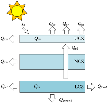
Figure 1. The proposed system SGSP-ORC
The SGSP is a basin filled with salted water and has a surface of 1000 m², a total depth of 3.25 m. The main parameters are reported in a subsequent table in the text (Table 2).
The ORC plant is fed by a heat exchanger placed in the LCZ. The heat removed by a process fluid, water, goes into the generator where the ORC working fluid is able to evaporate. The working fluids considered in this paper are R123 (2,2-Dichloro-1,1,1-trifluoroethane, HCFC group) and R245fa (1,1,1,3,3-Pentafluoropropane, HFC group), which are two suitable and available common fluids.
3.1 UCZ, upper convective zone
The energy balance for this layer (see Figure 2) is given as:
DUu = Qru + Qub - Quc - Qur - Que - Qwu (1)
Figure 2. The energy balance for the SGSP
where DUu is the internal energy stored in the UCZ, given as
$\Delta {{U}_{u}}={{\rho }_{u}}\,{{c}_{pu}}\,{{A}_{u}}\,{{X}_{u}}\,\frac{\text{d}{{T}_{u}}}{\text{d}t}$ (2)
The pond is supposed unburied and well insulated laterally, so each heat transfer to the wall may be neglected (Qwu = 0) [9]. This is also assumed for the NCZ and the LCZ layers (Qwl = Qwn = 0) [9].
3.1.1 The solar radiation in the SGSP
In order to obtain the rate of solar radiation absorbed by the UCZ, Qru, the Authors have considered relations reported in Duffie and Beckman [13] and Husain et al. [10].
Starting from available solar radiation data on a horizontal plane, the Authors calculate normal radiation utilizing the following procedure. They have used the equations for:
- the solar declination:
$\delta =23.45\ \sin \left( \frac{360\times (284+N)}{365} \right)$ (3)
where N is the number of the day in the year (1 … 365);
- the hour angle:
ω = 15 (j - 12) (4)
where j is the solar time in the day (0 … 23);
- incident angle:
Ji = cos-1[cos(Lat) cos(d) cos(ω) + sin(Lat) sin(d)] (5)
- normal radiation:
${{I}_{n}}=\frac{{{I}_{b}}}{\cos ({{\vartheta }_{i}})}$ (6)
while the reflective coefficient is calculated by following equation [14]:
$r=0.6\times {{\left( \frac{\sin ({{\vartheta }_{i}}-{{\vartheta }_{r}})}{\sin ({{\vartheta }_{i}}+{{\vartheta }_{r}})} \right)}^{2}}+0.4\times {{\left( \frac{\tan ({{\vartheta }_{i}}-{{\vartheta }_{r}})}{\tan ({{\vartheta }_{i}}+{{\vartheta }_{r}})} \right)}^{2}}$ (7)
Consequently, the solar radiation flux that enter inside the solar pond is equal to:
I0 = r × I0n (8)
while the available radiation at a depth x can be calculated by the following relation [15]:
${{I}_{x}}={{I}_{0}}\left\{ 0.36-0.08\ \ln \left( \frac{x}{\cos ({{\vartheta }_{r}})} \right) \right\}$ (9)
The radiation flux reaching the bottom is:
${{I}_{B}}={{I}_{0}}\left\{ 0.36-0.08\ \ln \left( \frac{L}{\cos ({{\vartheta }_{r}})} \right) \right\}$ (10)
where L is a depth of solar pond.
At the bottom, a certain part of radiation flux is absorbed by the bottom and the other part is reflected upwards.
If ζ is the reflectivity of the bottom, the reflected part is obtained as:
${{I}_{BR}}={{I}_{B}}\,\zeta \left\{ 0.36-0.08\ \ln \left( \frac{L-x}{\cos \,60{}^\circ } \right) \right\}$ (11)
Furthermore, the reflected radiation will travel towards solar pond surface and, at surface, a part of radiation will be reflected back towards bottom of solar pond. The surface reflects specularly and with a reflectivity towards inside equal to 0.477 [16]. In order of taking into account the contribution of this reflection, the last contribution is obtained as
${{I}_{SR}}=0.477\,{{I}_{B}}\,\zeta \left\{ 0.36-0.08\ \ln \left( \frac{L+x}{\cos \,60{}^\circ } \right) \right\}$ (12)
Therefore, Qru is given as:
Qru = (I0 + IBR,x=Xu + ISR,x=0) - (Ix=Xu + IBR,x=0 + ISR,x=Xu) (13)
3.1.2 The other terms of the energy balance
Qub is the heat transferred from bottom to top of the solar pond across the NCZ:
${{Q}_{ub}}=\frac{{{A}_{u}}({{T}_{s}}-{{T}_{u}})}{{{R}_{ncz}}}$ (14)
The thermal resistance of the NCZ is:
${{R}_{ncz}}=\frac{1}{{{h}_{1}}}+\frac{{{X}_{ncz}}}{{{k}_{w}}}+\frac{1}{{{h}_{2}}}$ (15)
Terms Quc, Qur, Que are the thermal losses to the internal energy stored in the UCZ. Quc is the convective heat transfer to the environment, given as:
Quc = hc Au (Tu - Ta) (16)
The convective heat transfer coefficient from the pond surface to the air is calculated with the McAdams formula [9], based on the average wind speed, v:
hc = 5.7 + 3.8 v (17)
Considering the emissivity of the water, e, assumed equal to 0.83 [9], Stefan-Boltzmann’s constant, s = 5.67 ×10⁻⁸ W/(m2 K4), and the sky temperature, Tk, the radiative heat transfer, Qur, is evaluated by the equation:
Qur =s e Au (Tu4 - Tk4) (18)
where the sky temperature is given as:
Tk = 0.0552 Ta1.5 (19)
Temperatures in Eq. (18) and Eq. (19) must be in kelvin.
The evaporative heat transfer from surface, Que, is given by Kishore and Joshi [17]:
${{Q}_{ue}}={{A}_{u}}\frac{\lambda \,{{h}_{c}}\,({{p}_{u}}-{{p}_{a}})}{1.6\,{{C}_{s}}\,{{p}_{atm}}}$ (20)
where Cs is the humid heat capacity of air, expressed as:
Cs = 1.005 + 1.82 gh [kJ/kg] (21)
The partial water vapour pressure pu at the upper layer temperature Tu is:
${{p}_{u}}=\exp \left( 18.403-\frac{3885}{{{T}_{u}}+230} \right)$ (22)
The partial water vapour pressure pa in the ambient temperature is:
${{p}_{a}}={{\gamma }_{h}}\,\exp \left( 18.403-\frac{3885}{{{T}_{a}}+230} \right)$ (23)
3.2 LCZ, lower convective zone
The energy balance for the LCZ (see Figure 2) is given as:
DUl = Qrs + Qub - Qground - Qload - Qwl (24)
where DUu is the internal energy stored in the UCZ, given as:
$\Delta {{U}_{l}}={{\rho }_{l}}\,{{c}_{pl}}\,{{A}_{l}}\,{{X}_{l}}\,\frac{\text{d}{{T}_{s}}}{\text{d}t}$ (25)
Qrs is the solar heat transferred from the overlying layers, and it may be calculated as previously done for the UCZ layer:
Qrs = (Ix=(Xu+Xncz) + ISR,x=(Xu+Xncz)) - (IBR,x=(Xu+Xncz)) (26)
Qground is the heat transferred from the pond to the ground. It is calculated as follows:
Qground = Kground Ab (Ts - Tg) (27)
where Kground is the overall heat transfer coefficient between the LCZ and the ground.
As aforementioned, the heat loss trough the wall is negligible (Qwl = 0). The term Qub is determined by Eq(14).
The term Qload represents the heat extracted that feeds the ORC system.
It has been here assumed that the system is installed on an area not shaded sited in the city of Palermo (38.12N, 13.34E - South of Italy).
4.1 Weather site description
The kind of climatic data set utilized for the simulation is the Test Referee Years (TRY), which provides hourly values of climatic parameters of the selected sites. The utilized climatic database is the Test Reference Year for the city of Palermo, in Italy [3].
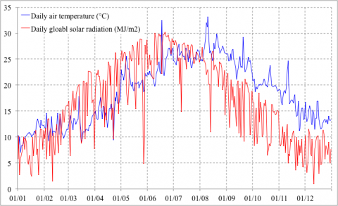
Figure 3. The trend of daily air temperature and daily global solar radiation of Palermo’s TRY
Figure 3 shows daily trends of air temperature and solar radiation for the site indicated.
Other input values were taken from technical and commercial literatures.
4.2 Selection of working fluids for the ORC
The working fluid is an important component of ORC system. In this work, two working fluids were compared in order to assess the potentiality of each of them for this application.
Table 1 shows the main thermophysical properties of the working fluid used in this work.
Table 1. Main thermophysical properties of the working fluid
|
Substance |
Molecular mass |
Tcrit |
pcrit |
Tbp |
ODP |
GWP |
|
|
[kg/kmol] |
[°C] |
[MPa] |
[°C] |
|
[100 year] |
|
R123 |
152.93 |
183.68 |
3.67 |
27.82 |
0.02 |
77 |
|
R245fa |
134.05 |
154.01 |
3.64 |
15.14 |
0 |
950 |
4.3 Simulation
The Authors have been implemented in the Python environment the mathematical model of the system in order to simulate the behavior of the above described ORC system fed by SGSP, considered as a quasi-static process.
The main parameters of the SGSP for the simulation are reported in Table 2.
It is supposed a solar pond with vertical wall, so that the area at upper and bottom layers is the same (Au = Al = Ab = A).
The thermophysical properties of the working fluids are calculated by means of the REFPROP [18]. The values of the most relevant parameters of the system were based on the current pertinent literature, since Wang et al. [19] did not provide complete information about their system. Moreover, flow rates are steady-state and, therefore, are not optimized; additionally, the system is characterized by an on-off operation mode. The pump and turbine isentropic efficiency were assigned as 70%. Furthermore, the flow rate in ORC varies in order of having always the temperature of 60 °C at the evaporator outlet in hot side. The condensing temperature is assumed equal to 25 °C.
Table 2.The main parameters of SGSP
|
Parameter |
value |
|
Depth of SGSP, L |
3.25 m |
|
Depth of UCZ, Xu |
0.70 m |
|
Depth of LCZ, Xl |
1.20 m |
|
Depth of NCZ, Xncz |
1.35 m |
|
Area of solar pond, A |
1000 m2 |
|
Water density, ru |
1000 kg/m3 |
|
Brine density, rl |
1200 kg/m3 |
|
Specific heat capacity of water in UCZ, cpu |
4180 J/(kg K) |
|
Specific heat capacity of water in LCZ, cpl |
3300 J/(kg K) |
|
Convective heat transfer coefficient between NCZ and UCZ, h1 |
56.58 W/(m2 K) |
|
Convective heat transfer coefficient between LCZ and NCZ, h2 |
48.28 W/(m2 K) |
|
Convective heat transfer coefficient between LCZ and surface at bottom, h3 |
78.12 W/(m2 K) |
|
Heat transfer coefficient from the outside surface to the atmosphere, h0 |
5.43 W/(m2 K) |
|
Thermal conductivity of water, kw |
0.596 W/(m K) |
|
Overall heat transfer coefficient, Kground |
0.4254 W/(m2 k) |
|
Latent heat of vaporization |
2257 kJ/kg |
Table 3. Turbine inlet temperature and pressure
|
Substance |
TT |
pT |
|
|
[°C] |
[MPa] |
|
R123 |
60.85 |
0.2859 |
|
R245fa |
60.85 |
0.4626 |
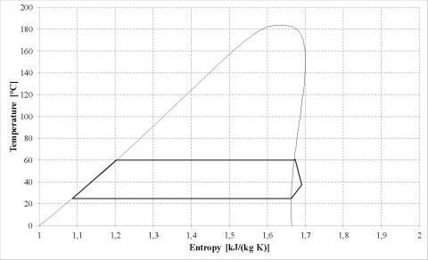
Figure 4. The ORC cycle for R123 fluid
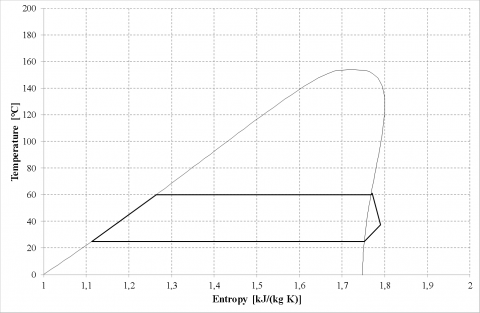
Figure 5. The ORC cycle for R245fa fluid.
Moreover, the Authors have utilized the values of turbine inlet temperature and pressure suggested by Wang et al. [19], reported in Table 3, with the reduction of 9 °C for the inlet temperature.
The ORC cycle, used in this work, has been reported in Figure 4 for R123 fluid and Figure 5 for R245fa.
The simulation has been carried out for two years for evaluating the effective production of energy by solar pond, in order to avoid the transient period, therefore the second year only has been investigated.
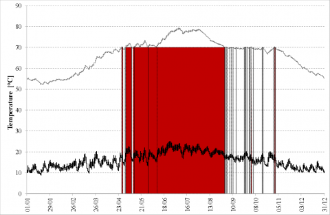
The trend of temperatures in UCZ layer, Tu, and in LCZ layer, Ts, is reported in Figure 6.
The Table 4 shows the first results for a simulation of the year investigated.
The annual average efficiency of solar pond has been assessed as the ratio between the annual heat extracted by the LCZ layer and the annual solar radiation flux within the salted water at surface of the pond. The assessed value is equal to 5.05%.
Figure 6. Trend of Temperature in UCZ and LCZ. In red the periods of working of ORC
Table 4. Results of simulations
|
Substance |
Pump consumption |
Turbine power output |
$\eta$ |
|
|
[kWh] |
[kWh] |
[%] |
|
R123 |
79 |
5561 |
6.7 |
|
R245fa |
131 |
5508 |
6.6 |
The SGSP is a technology that is currently very interesting and many researchers are investigating on it. It requires wide and available area due to the low energetic density.
Therefore, this technology is appropriate for countries with a low electrification level and with a large amount of unutilized land.
The study here conducted with a coupling of a SGSP and an ORC with two of the fluids more investigated at the moment (R123 and R245fa) shows that the efficiencies are aligned with the main results in Literature.
The results show, as pertains the efficiencies, a substantial equality of value among the fluids. Deep considerations must be carried on regards the environmental aspects, and with the plants programming. In fact, the end of production of Refrigerant 123 is scheduled by 2030, due the ODP correlated, despite the R245fa that, on the other side, has an elevated GWP value.
|
A |
area (m²) |
|
Ab |
area of the bottom surface of the pond (m²) |
|
Al |
surface area of the LCZ (m²) |
|
Au |
surface area of the UCZ (m²) |
|
cpl |
heat capacity of water in LCZ (J/kg K) |
|
cpu |
heat capacity of water in UCZ (J/kg K) |
|
Cs |
humid heat capacity (kJ/kg K) |
|
h0 |
heat transfer coefficient from the outside surface to the atmosphere (W/m² K) |
|
h1 |
heat transfer coefficient between the NCZ and the UCZ (W/m² K) |
|
h2 |
heat transfer coefficient between the LCZ and the NCZ (W/m² K) |
|
h3 |
heat transfer coefficient between the LCZ with surface at the bottom of the SGSP (W/m² K) |
|
hc |
convective heat transfer coefficient to the air (W/m² K) |
|
I |
solar radiation (W/m²) |
|
Kground |
overall heat transfer coefficient to the ground (W/m² K) |
|
kw |
thermal conductivity of water (W/m K) |
|
L |
depth of SGSP (m) |
|
Lat |
Latitude (degree) |
|
LCZ |
Lower Convective Zone |
|
N |
number of the day |
|
NCZ |
NonConvective Zone |
|
p |
pressure (MPa) |
|
pa |
the partial pressure of water vapour in the ambient temperature (mmHg) |
|
patm |
atmospheric pressure (mmHg) |
|
pu |
water vapour pressure at the upper layer temperature (mmHg) |
|
Qground |
heat loss to the ground (W/m²) |
|
Qload |
heat extracted from the LCZ (W/m²) |
|
Qri |
solar radiation entering the UCZ (W/m²) |
|
Qrs |
solar radiation entering and stored in the LCZ (W/m²) |
|
Qru |
solar radiation that is absorbed in the UCZ (W/m²) |
|
Qub |
conduction heat transfer to the UCZ (W/m²) |
|
Quc |
convective heat loss from UCZ (W/m²) |
|
Que |
evaporative heat loss from UCZ (W/m²) |
|
Qur |
radiation heat loss from UCZ (W/m²) |
|
Qwu, Qwn, Qwl |
heat loss through walls of the pond, resp. from UCZ, NCZ and LCZ (W/m²) |
|
r |
reflective coefficient |
|
Rncz |
thermal resistance of NCZ (m² K/W) |
|
t |
time (s) |
|
T |
temperature (°C) |
|
Ta |
average of the ambient temperature (°C) |
|
Tg |
temperature of the ground under the SGSP (°C) |
|
Tk |
sky temperature |
|
Ts |
temperature of the LCZ (°C) |
|
Tu |
temperature of the UCZ (°C) |
|
U |
internal energy (W/m²) |
|
UCZ |
Upper Convective Zone |
|
v |
monthly average wind speed (m/s) |
|
Xncz, Xl, Xu |
thickness of the NCZ, LCX and UCZ respectively (m) |
|
Greek symbols |
|
|
$\delta$ |
solar declination (degree) |
|
$\varepsilon$ |
emissivity of water |
|
$\lambda$ |
latent heat of vaporisation (kJ/kg) |
|
$\sigma$ |
Stefan–Boltzmann’s constant |
|
$\gamma_{h}$ |
relative humidity |
|
$\rho_{l}$ |
density of the LCZ(kg/m³) |
|
$\rho_{u}$ |
density of the UCZ (kg/m³) |
|
$\omega$ |
hour angle (degree) |
|
$\varphi$ |
solar time (h) |
|
$\eta$ |
efficiency |
|
$\vartheta_{i}$ |
incident angle (degree) |
|
Subscripts |
|
|
B |
bottom |
|
bp |
boiling point |
|
crit |
critical values |
|
l |
LCZ |
|
n |
normal |
|
R |
reflected |
|
S |
surface |
|
T |
turbine |
|
u |
UCZ |
|
x |
Generic depth |
[1] OECD (2016), Executive Summary, World Energy Outlook 2016, IEA, Paris. http://dx.doi.org/10.1787/weo-2016-2-en
[2] Ranjan K.R., Kaushik S.C. (2014). Thermo-dynamic and economic feasibility of solar ponds for various thermal applications: A comprehensive review, Renewable and Sustainable Energy Reviews, Vol. 32, pp. 123-139. DOI: 10.1016/j.rser.2014.01.020
[3] Sorrentino G., Scaccianoce G., Morale M., Franzitta V. (2012). The importance of reliable climatic data in the energy evaluation, Energy, Vol. 48, No. 1, pp. 74-79. DOI: 10.1016/j.energy.2012.04.015
[4] El-Sebaii A.A., Ramadan M.R.I., Aboul-Enein S., Khallaf A.M. (2011). History of the solar ponds: A review study, Renewable and Sustainable Energy Reviews, Vol. 15, No. 6, pp. 3319-3325. DOI: 10.1016/j.rser.2011.04.008
[5] Berkani M., Sissaoui H., Abdelli A., Kermiche M., Barker-Read G. (2015). Comparison of three solar ponds with different salts through bi-dimensional modeling, Solar Energy, Vol. 116, pp. 56-68. DOI: 10.1016/j.solener.2015.03.024
[6] Hordeski M.F. (2004). Dictionary of Energy Efficiency Technologies, Lilburn, Georgia, The Fairmont Press, USA, pp. 245-246.
[7] Ding L.C., Akbarzadeh A., Date A. (2016). Electric power generation via plate type power generation unit from solar pond using thermoelectric cells, Applied Energy, Vol. 183, pp. 61-76. DOI: 10.1016/j.apenergy.2016.08.161
[8] Ziapour B.M., Saadat M., Palideh V., Afzal S. (2017). Power generation enhancement in a salinity-gradient solar pond power plant using thermoelectric generator, Energy Conversion and Management, Vol. 136, pp. 283-293. DOI: 10.1016/j.enconman.2017.01.031
[9] Sayer A.H., Al-Hussaini H., Campbell A.N. (2016). New theoretical modelling of heat transfer in solar ponds, Solar Energy, Vol. 125, pp. 207-218. DOI: 10.1016/j.solener.2015.12.015
[10] Husain H., Patil S.R., Patil P.S., Samdarshi S.K. (2004). Simple methods for estimation of radiation flux in solar ponds, Energy Conversion and Management, Vol. 45, No. 2, pp. 303-314. DOI: 10.1016/S0196-8904(03)00122-5
[11] Abbassi Monjezi A., Campbell A.N. (2016). A comprehensive transient model for the prediction of the temperature distribution in a solar pond under Mediterranean conditions, Solar Energy, Vol. 135, pp. 297-307. DOI: 10.1016/j.solener.2016.06.011
[12] La Gennusa M., Morale M., Peri G., Rizzo G., Scaccianoce G. (2015). Organic rankine cycle fed by flat-plate solar collectors: A case study, Proc. 9th Nat. Conf. AIGE, Catania, Italy.
[13] Duffie J.A., Beckman W.A. (2013). Solar Engineering of Thermal Processes, 4th ed. Hoboken, New Jersey, USA.
[14] Hawlader M.N.A. (1980). The influence of the extinction coefficient on the effectiveness of solar ponds, Solar Energy, Vol. 25, No. 5, pp. 461-464. DOI: 10.1016/0038-092X(80)90454-5
[15] Bryant H.C., Colbeck I. (1977). A solar pond for London, Solar Energy, Vol. 19, No. 3, pp. 321-322. DOI: 10.1016/0038-092X(77)90079-2
[16] Cengel Y.A., Özişik M.N. (1984). Solar radiation absorption in solar ponds, Solar Energy, Vol. 33, No. 6, pp. 581-591. DOI: 10.1016/0038-092X(84)90014-8
[17] Kishore V.V.N., Joshi V. (1984). A practical collector efficiency equation for nonconvecting solar ponds, Solar Energy, Vol. 33, No. 5, pp. 391-395. DOI: 10.1016/0038-092X(84)90190-7
[18] Lemmon E.W., Huber M.L., McLinden M.O. (2013). NIST Standard Reference Database 23: Reference Fluid Thermodynamic and Transport Properties-REFPROP, Version 9.1, NIST - National Institute of Standards and Technology, Standard Reference Data Program, Gaithersburg, Maryland, USA.
[19] Wang M., Wang J., Zhao Y., Zhao P., Dai Y. (2013). Thermodynamic analysis and optimization of a solar-driven regenerative organic Rankine cycle (ORC) based on flat-plate solar collectors, Applied Thermal Engineering, Vol. 50, No. 1, pp. 816-825. DOI: 10.1016/j.applthermaleng.2012.08.013