Modeling the interaction of coolant flows at the liquid-solid boundary with allowance for the laminar boundary layer

In the current energy crisis, the issue of energy efficiency of heat exchange processes and equipment for their provision in food, chemical, pharmaceutical, processing and other technologies becomes decisive. To increase the heat transfer coefficients in heat exchangers, various methods are used, in particular, the modification of the structural elements of boilers and other equipment [1], the increase in the turbulence of the refrigerant flows [2], the use of liquids with the optimal concentration of surfactants (SAS). For example, the maximum rate of heat exchange was observed when a nonionic surfactant was added to water [3]. The authors of [3] believed that the maximum rate of heat exchange in the first place may be due to the fact that this additive has a minimum capacity for the formation of foam. In addition, it is known that surface-active substances significantly, approximately 2 times, reduce the coefficients of surface tension of water and other liquids.

3.1. Analysis of the forces in LBL

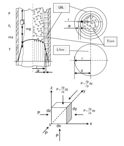
It is common knowledge that for the pipeline, and in particular for tubes heat exchangers the vectors of flow average velocities are distributed in tube longitudinal section as a parabola (Fig. 1).

At the boundary of the flow of a liquid and a pipe there is always a LBL [9]. This layer has a very small average thickness, but its effect on heat transfer and diffusion processes that occur in the flow is crucial. Consider the elementary volume of liquid in the pipeline within the limits LBL (Fig. 1.)

1.png

Figure 1. Forces acting on an elementary volume of liquid in LBL

On elementary volume of liquid in LBL is acted upon by forces:

1. Force of surface tension of liquid:                                                                                                  $F_{\sigma}=2 \pi(d x) \cos \theta \sigma$;     (1)

2. Force of gravity:                                                                                                                           $m g=\rho g(d x d y d z)$;      (2)

3. Friction force:                                                                                                                          $T=\mu \frac{d^{2} V_{z}}{d z^{2}}(d x d y d z)$;        (3) 

4. Force of inertia:                                                                                                        $F_{i}=m a=\rho \frac{d V_{z}}{d \tau}(d x d y d z)$;        (4)

5. Force of pressure:                                                                                                           $P=-\frac{d \mathrm{p}}{d \mathrm{z}}(d x d y d z)$,       (5)

where, P – fluid pressure acting on the upper face of the elementary volume, Pa; $V_{z}$ – average fluid velocity in LBL,  m/s; $\sigma$ – the surface tension of the liquid, N/m; ρ – fluid density, kg/m³; g – acceleration of gravity, m/s²;  μ – coefficient of dynamic viscosity, N.s/m²; $\tau$ – time, s; cosq  – cosine of wetting angle;

According to the principle of d'Alembert, the algebraic sum of all forces acting on the elementary volume is equal to the force of inertia. When dividing by (dxdydz), we get the equation 6. This is the Navier-Stokes equation, which is supplemented by surface forces, which according to our statement in LBL reach commensurate values with pressure forces:

$\frac{2 \pi(d x) \sigma \cos \theta}{(d x d y d z)}+\rho g-\frac{d P}{d z}+\mu \frac{d^{2} V_{z}}{d z^{2}}=\rho \frac{d V_{z}}{d \tau}$     (6)

Equation 6 can not be integrated, so we obtain a number equation from it, applying the similarity theory. The symbols of differentiation of the differential equation and direction are removed, we replace the linear parameters of the elementary volume dx, dy, dz by l.

Based on the similarity theory, taking into account that the fluid velocity and the linear parameter l inside LBL are very small, dividing the right and left sides of equation (6) by$\rho V_{Z / \tau}$, we get the numbers:  we get the numbers: 

1. $\frac{2 \pi \sigma \cos \theta \tau}{\rho V_{z} l^{2}}=\frac{2 \pi \sigma \cos \theta \mu}{\rho V_{z}^{2} l \mu}=\frac{1}{N} \frac{2 \pi \sigma \cos \theta}{\mu V_{z}}$= Pо– supface number in LBL     (7)

where N – modified Reynolds number in LBL $N=\frac{\rho V_{z} l}{\mu} \approx 10,47-11,5[10]$ [10]; 

2. $\frac{p \tau}{\rho V_{z} l}=\frac{\Delta p}{\rho V_{z}^{2}}=E u$ – Euler number in LBL      (8)

3.$\frac{\rho g \tau}{\rho V_{z}}=\frac{g \tau l}{V_{z} l}=\frac{g l}{V_{z}^{2}}=F r$ – Froude number in LBL     (9) 

4.$\frac{\mu V_{z} \tau}{l^{2} \rho V_{z}}=\frac{\mu}{l \rho V_{z}}=\frac{1}{\operatorname{Re}}$ –  Reynolds number in LBL     (10)

We substitute in the numbers 1, 2, 3, 4 characteristics of water under normal conditions: $\Delta P \approx 100000$ Pа – decline in pressure in the pipeline; ρ ≈ 1000 fluid density, kg/m³; $V \approx 1$ m/s – the average velocity of liquids in pipelines; $V_{z} \approx \frac{V}{10} \approx 0.1$[10] m/s – the average velocity of liquids in LBL; $\sigma \approx 0.0725$ N/m – the surface tension of the water under normal conditions, N/m;  cos θ ≈ 0,8 – cosine of wetting angle; $\mu \approx 1 \cdot 10^{-3}$– coefficient of dynamic viscosity, N.s/m²; δ ≈ 0.3×10^-3 m – average thickness LBL under turbulent driving condition of water in the pipes.

1. $P o=\frac{1}{\mathrm{N}} \frac{2 \pi \cdot \sigma \cdot \cos \theta}{\mu V_{z}} \approx \frac{1}{10.5} \frac{2 \cdot 3.14 \cdot 0.0725 \cdot 0.8}{1 \cdot 10^{-3} \cdot 0.1} \approx 347$ 

2.  $E u=\frac{\Delta p}{\rho V_{z}^{2}} \approx \frac{100000}{1000 \cdot(0.1)^{2}} \approx 10000$;

3. $F r=\frac{g \cdot l}{V_{z}^{2}} \approx \frac{10 \cdot \delta}{(0.1)^{2}} \approx \frac{10 \cdot 0.3 \cdot 10^{-3}}{(0.1)^{2}} \approx 0.3$;   

4. $\frac{1}{\mathrm{Re}}=\frac{\mu}{\delta \rho V_{z}} \approx \frac{10^{-3}}{0.3 \cdot 10^{-3} \cdot 1000 \cdot 0.1} \approx 0.03$;

The Froude number and the inverse Reynolds number are 4-5 orders of magnitude smaller than the surface criterion and the Euler number in the laminar boundary layer, which allows neglecting the forces of gravity and friction in these conditions.

3.2 The formula for calculating the average thickness of LBL

Consider the pressure force and force of surface tension in laminar boundary layer actings in the elementary ring of liquid (Fig. 1):

- the area of elementary ring: $d A=2 \pi r d r$;

- the pressure force acting on elementary ring of the laminar boundary layer: $d P=\Delta P 2 \pi r d r$;

- the force of surface tension acting on elementary ring in the laminar boundary layer: $F_{\sigma}=2 \pi \sigma \cos \theta d r$;

Taking into account only the pressure forces and the forces of surface tension, we integrate the equation changing the limits of integration r and $\delta$.

The physical meaning of integration in this system is that the laminar boundary layer covers the entire passage of the pipeline, the boundary of the transition laminar-turbulent, have the limiting case-the average thickness of the laminar boundary layer is equal to the radius of the tubes $\delta=r=\frac{d}{2}$ (Fig. 1).

$P=\Delta P 2 \pi \int_{0}^{\delta} r d r=\pi \Delta P \delta^{2}$;

$d F_{\sigma}=2 \pi \sigma \cos \theta \int_{0}^{r} d \delta=2 \pi \sigma \cos \theta r$;

Based on the principle of theoretical fluid mechanics, after integration and reduction of the number π, we get equation (11):

$\delta=\sqrt{\frac{\sigma d \cos \theta}{\Delta P}}$.     (11)

Formula (11) describes the flow of liquid at the boundary of the laminar and transient flow of liquid flow at a critical Reynolds number Re_cr = 2320. For Reynolds number values that are greater than the critical values in equation (11) introduced the coefficient of turbulence К_Т   (12).

$\delta=\frac{\sqrt{\frac{\sigma \cos \theta d}{\Delta P}}}{K_{T}}$ ,      (12)

К_Т – the coefficient of turbulence, $K_{T}=\frac{R e}{R e_{c r}}$.

One should notice that for the boundary conditions, when the pipe is reduced to the capillary size, i.e. the diameter d becoming small, the equation (12) transforms into the Laplace’s equation $\Delta P=\frac{4 \sigma \cos \theta}{d}$; (at $\delta=r=\frac{d}{2}$; $\frac{d^{2}}{4}=\frac{\sigma d \cos \theta}{\Delta P}$); It is obvious that in the capillary goes laminar fluid motion mode. Therefore, the ratio $\frac{R e}{R e_{c r}}=1$. 

If write the difference of pressure in accordance with Darcy’s equation and make conversions, from equation (12) we obtain the equation (13):

$\delta=\frac{\frac{d^{2}}{\operatorname{Re} \mu} \sqrt{\frac{2 \sigma \cos \theta \rho}{f L}}}{\frac{\operatorname{Re}}{\operatorname{Re}_{c r}}}$     (13)

where ΔP – pressure drop along the pipe or apparatus, Pa;

r – the radius of elementary ring, m; f – Darcy coefficient;

ρ – fluid density, kg/m³; L – length of the pipe, m;

d – diameter of the pipe, m; cosθ – the cosine of the contact angle; δ – the average thickness of the laminar boundary layer, m; $\cos \theta$ – the surface tension of the liquid, N/m; µ – coefficient of dynamic viscosity, N.s/m²; Re – the Reynolds number; Re_cr – the critical Reynolds number $\left(R e_{c r}, \approx 2320\right)$; 

V – the velocity of the fluid flow, m/s.

3.3 Effect of surfactants on the average thickness of LBL

The resulted ratios (12, 13) shows that the average thickness LBL marginally depends on the coefficient of fluid dynamic viscosity. And it is not unexpected, because the friction forces in laminar boundary layer are very small due to the very lows sliding velocity of adjacent layers. However, the average thickness the laminar boundary layer depends on the surface tension coefficient and of the cosine of the contact.

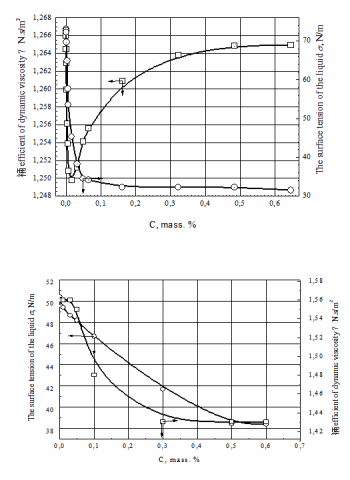
Equation (7) shows that the numerical values of the surface criterion depend substantially on the surface tension coefficient. It is known that the coefficient of surface tension of liquid-phase heat carriers can be reduced by introducing optimal concentrations of SAS. To the aqueous solutions (model fluid 1) we added the most common non-ionic SAS. As a surfactant for the components of milk (model liquid 2) - vegetable oil of pumpkin. To determine the range of values of the surface criterion, a series of experiments was performed to ensure changes in the coefficient of surface tension, the cosine of the wetting angle, and the dynamic coefficient of viscosity of aqueous solutions and milk under the influence of SAS, which were measured according to well-known procedures. 

In Fig. 2 shows the dependence of the surface tension coefficient, the dynamic coefficient of viscosity of the water (a) and milk (b) wetting angle on the SAS concentrations. As can be seen from the graphs, the curve of the dependence of the surface tension on the concentration has minima close to the critical concentration of micelle (CCM) formation. That is, with a slight increase in surfactant concentrations, the surface tension coefficient decreases sharply to the CCM, and at a concentration above the CCM, its decrease is insignificant. For non-ionic SAS the CCM is observed at a concentration (0.05 … 0.10) by mass. %. At the same time, the coefficient of surface tension decreases by 2.32 times in comparison with water.

As can be seen from the graphs, the minimum value of the surface tension coefficient of milk is observed at a concentration (0.5…0.6) by mass. % pumpkin oil. These concentrations SAS were considered optimal. At these SAS concentration, the value for the dynamic viscosity coefficient was also selected.

Let us show the change in the surface number in LBL for aqueous solutions with the addition of the optimum concentrations of the surfactants studied. The rate in LBL was determined from the modified Reynolds number, taking the value N = 10.5, and the average thickness of the LBL was found from the formula (13). In the food, pharmaceutical and processing industries, the average fluid velocity in heat exchange equipment is $V \approx 1 m / s$, pipe diameter d = 21·10^-3 m, pipe length L=3 m.

2.png

Figure 2. Dependence of the coefficient of surface tension and the dynamic coefficient of viscosity on the concentration of surfactants (а) water from the concentration of non-ionic SAS, (b) milk from the concentration of pumpkin oil.

The results of calculations are presented in Table 1.

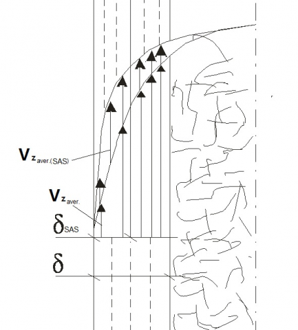
Let us consider the cross section of the flow in a pipeline under the turbulent (T) regime of fluid motion (Fig. 3). The velocity vectors in it are distributed like a parabola, but with a wider vertex.

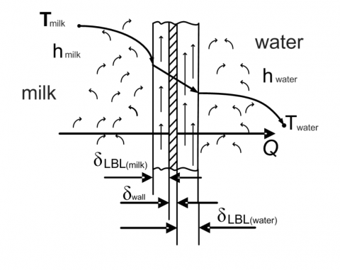
Reducing the average thickness LBL of water and milk, the speed in them increases, and this intensifies the passage of the amount of heat through it (Fig. 4).

Table 1. The value of the surface number at the optimum surfactant concentrations in the model fluid 1  (“ice” water) and in the model fluid 2 (milk)

3.png

Figure 3. Medium velocity vectors in LBL without SAS and with using SAS

4.png

Figure 4. Heat transfer scheme Q through the metal wall from milk to water