OPEN ACCESS
This paper develops a water holdup calculation model based on flow characteristics for no-slip oil-water two phase flow. The model is constructed in consideration of two flow patterns: the stratified flow (ST) and the stratified flow with some mixing at the interface (ST&MI). The predicted values obtained by the model are compared with the test data on white oil-water flow. The results show that the model can accurately predict the water holdup of no-slip oil-water two-phase flow, which is of great significance for the determination of the working parameters in oilfields.
oil-water two-phase flow, no-slip water holdup, inlet water fraction, stratified flow model,three-phase segregated flow model
The research of oil-water flow has direct bearing on the economic design and operation in oilfields [1] as 1/3 of the total investment on surface engineering goes to oil pipelines and 40% of the total energy consumption of production takes place during transportation.
The oil-water two-phase flow is a common phenomenon in the oil industry. When the oil is finally delivered, the oil and water are immiscible with each other and have significant differences in density. During the movement in well bores or pipelines, the oil and water slip past each other owing to the velocity difference. The smaller the slippage velocity between oil and water, the lower the pressure loss of the oil-water two- phase flow. Thus, the research of water holdup in no-slip oil- water two-phase flow can laya theoretical basis for identifying the working parameters in oil gathering and transmission systems.
For horizontal pipes, the water holdup in oil-water two-phase flow is greatly affected by the flow pattern. Even with identical inlet water fraction, the water holdup may differ depending on the flow pattern in the pipe. Since the 1950s,much research has been done to understand the flow pattern of the oil-water two-phase flow. For this purpose, a series of experiments were conducted by Russell [2] (1959), Charles [3] (1961), Guzhov [4] (1973), Malinowsky [5] (1975),Oglesby [6] (1979), Martinez [7] (1983), and Arirachakaran [8] (1989), to name but a few. From 1990 onward, the following scholars realized more accurate measurement of various parameters of flow patterns, and objective analysis of the flow patterns of oil-water two-phase flow thanks to the advancement of instrument and technology: Trallero[9](1995), Trallero and Brill [10] (1996), Nadler and Mewes [11](1997), Angeli and Hewitt [12] (1998), Shi and Jepson [13](1999), Angeli and Hewitt [14] (2000), Chen Jie [15~17](2000~2003), Shi [18] (2001), Yao Haiyuan and Gong Jing[19~20] (2004~2006), Al-Wahaibi [21~24] (2007~2012),M Castro[25] (2014), and Al-Sarkhi [26] (2017). According to Trallero (1995), the oil-water two-phase flow patterns could be classified into two categories: the segregated flows(ST; ST&MI) and dispersed flows (Do/w&w; O/w;Dw/o&Do/w; W/o). In the dispersed flows, the oil and water are expected to be fully mixed and the degree of homogenization is so high that the oil-water slippagevelocity reaches zero. Besides, the Do/w&w pattern is only reported twice in Valle and Kvandal. (1995), Nadler and Mewes et al.(1997). Therefore, only the stratified flow (ST) and stratified flow with interfacial mixing (ST&MI) are taken into account in this research.
2.1 The ST model
The momentum balance in the oil layer and the water layer of the ST is expressed as follows.In the oil layer:
$-\frac{d p}{d x} A_{o}-\tau_{o} S_{o} \pm \tau_{i} S_{i}+A_{o} \rho_{o} g \sin \alpha=0$ (1)
In the water layer:
$-\frac{d p}{d x} A_{w}-\tau_{w} S_{w} \mp \tau_{i} S_{i}+A_{w} \rho_{w} g \sin \alpha=0$ (2)
Assume at the two layers share the same pressure drop, and cancel out the pressure drop terms in (1) and (2).
$\tau_{o} \frac{S_{o}}{A_{0}} \mp \tau_{l}\left(\frac{S_{i}}{A_{o}}+\frac{S_{i}}{A_{w}}\right)-\tau_{w} \frac{S_{w}}{A_{w}}+\left(\rho_{w}-\rho_{o}\right) g \sin \alpha=0$ (3)
In a horizontal pipe, the inclination angle of the pipe α=0o.If the slippage velocity is 0, then Uo = Uw.
The shear stress of the two layers are evaluated by a Blasius-type equation (Taitel and Dukler, 1976) [27]:
$\tau_{o}=f_{o} \rho_{o} \frac{U_{o}^{2}}{2}$ (4)
$\tau_{w}=f_{w} \rho_{w} \frac{U_{w}^{2}}{2}$ (5)
The shear stress of phase interface is obtained by the following equation:
$\tau_{i}=f_{i} \frac{\rho\left(U_{o}-U_{w}\right)^{2}}{2}(\rho=\text { the density of the faster phase })$ (6)
where the friction factors are evaluated by the Brauner’sapproach [28] (1989):
$f_{o}=C_{o}\left(\frac{D_{o} U_{o} \rho_{o}}{\mu_{o}}\right)^{-n_{o}}$ (7)
$f_{w}=C_{w}\left(\frac{D_{w} U_{w} \rho_{w}}{\mu_{w}}\right)^{-n_{w}}$ (8)
$f_{i}=B f_{w} \quad\left(U_{w}>U_{o}\right)$ (9)
$f_{i}=B f_{o} \quad\left(U_{w}<U_{o}\right)$ (10)
$f_{m}=C_{m}\left(\frac{D_{m} U_{m} \rho_{m}}{\mu_{m}}\right)^{-n_{m}}$ (11)
Substitute Equations (4)~(10) into (3), and we have
$C_{o}\left(\frac{D_{o} U_{o} \rho_{o}}{\mu_{o}}\right)^{-n_{s}} \rho_{o} \frac{S_{o}}{A_{o}}=C_{w}\left(\frac{\left.D_{w} U_{w} \rho_{w}\right)}{\mu_{w}}\right)^{-n_{w}} \rho_{w} \frac{S_{w}}{A_{w}}$ (12)
where the values of the coefficients Co, w and no, w depend on the specific flow pattern.
For turbulent flow, Co, w=0.046 and no, w=0.2. In this case, Equation (12) can be rewritten as:
$\left(\frac{D_{o} U_{o} \rho_{o}}{\mu_{o}}\right)^{-0.2} \rho_{o} \frac{S_{o}}{A_{o}}=\left(\frac{\left.D_{w} U_{w} \rho_{w}\right)}{\mu_{w}}\right)^{-0.2} \rho_{w} \frac{S_{w}}{A_{w}}$ (13)
where the hydraulic equivalent diameter is expressed as:
$D_{o}=\frac{4 A_{o}}{\left(S_{o}+S_{l}\right)} \quad D_{w}=\frac{4 A_{w}}{S_{w}}\left(U_{o}>U_{w}\right)$ (14)
$D_{o}=\frac{4 A_{o}}{S_{o}} \quad D_{w}=\frac{4 A_{w}}{\left(S_{w}+S_{l}\right)}\left(U_{o}<U_{w}\right)$ (15)
$D_{o}=\frac{4 A_{o}}{S_{o}} \quad D_{w}=\frac{4 A_{w}}{S_{w}}\left(U_{o} \approx U_{w}\right)$ (16)
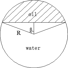
Figure 1. Sketch map of the wetted perimeter in the oil-water ST
As shown in Figure 1, the wetted perimeter and the cross- sectional area of the pipe are calculated as:
$S_{o}=2 R \beta$ (17)
$S_{w}=2 R(\pi-\beta)$ (18)
$A_{o}=R^{2} \beta-\frac{1}{2} R^{2} \sin 2 \beta$ (19)
$A_{w}=R^{2}(\pi-\beta)+\frac{1}{2} R^{2} \sin 2 \beta$ (20)
Substitute Equations (16)~(20) into (13), and we have:
$\left(\frac{\mu_{o} \rho_{o}^{4}}{\mu_{w} \rho_{w}^{4}}\right)^{\frac{1}{6}} \frac{S_{o}}{S_{w}}=\frac{A_{o}}{A_{w}} \Leftrightarrow\left(\frac{\mu_{o} \rho_{o}^{4}}{\mu_{w} \rho_{w}^{4}}\right)^{\frac{1}{6}} \frac{\beta}{\pi-\beta}=\frac{2 \beta-\sin 2 \beta}{2(\pi-\beta)+\sin 2 \beta}$ (21)
For the ST, the inlet water fraction and water holdup are equal. Thus, theinlet water fraction is:
$\eta_{w}=\frac{2(\pi-\beta)+\sin 2 \beta}{2 \pi}$ (22)
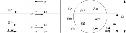
2.2 The three-phase segregated flow model
When it comes to the ST&MI, Vedapuri (1997) [3] developed a three-layer flow model for predicting the water film in oil-water two-phase flow. The model treats the oil layer, water layer and mixed layer as three different phases with distinctive properties. Thus, the oil-water two-phase flow is converted to a three-phase stratified flow of oil,mixture and water. Figure 2 shows the sketch map of this model.
Figure 2. Sketch map of the three-phase segregated flow In the water layer:
$-A_{w}\left(\frac{d p}{d x}\right)-\tau_{w} S_{w}+\tau_{i 1} S_{i 1}-\rho_{w} A_{w} g \sin \alpha=0$ (23)
In the mixture layer:
$-A_{m}\left(\frac{d p}{d x}\right)-\tau_{m} S_{m}-\tau_{i 1} S_{i 1}+\tau_{i 2} S_{i 2}-\rho_{m} A_{m} g \sin \alpha=0$ (24)
In the oil layer:
$-A_{o}\left(\frac{d p}{d x}\right)-\tau_{o} S_{o}-\tau_{i 2} S_{i 2}-\rho_{o} A_{o} g \sin \alpha=0$ (25)
Cancel out the pressure drop terms in (23) and (24), and we have:
$\tau_{m} \frac{S_{m}}{A_{m}}-\tau_{w} \frac{S_{w}}{A_{w}}-\tau_{i 2} \frac{S_{i 2}}{A_{m}}+\tau_{i 1}\left(\frac{S_{i 1}}{A_{m}}+\frac{S_{i 1}}{A_{w}}\right)+\left(\rho_{m}-\rho_{w}\right) g \sin \alpha=0$ (26)
Similarly, the following equation is established based on (24) and (25):
$\tau_{o} \frac{S_{o}}{A_{o}}-\tau_{m} \frac{S_{m}}{A_{m}}-\tau_{i 1} \frac{S_{i 1}}{A_{m}}+\tau_{i 2}\left(\frac{S_{i 2}}{A_{o}}+\frac{S_{i 2}}{A_{m}}\right)+\left(\rho_{o}-\rho_{m}\right) g \sin \alpha=0$ (27)
In a horizontal pipe, a = 0°.
The three-phase segregated flow model hypothesis by Vedapuri et al. (1997) suggests that, in the case of low oil viscosity, the water holdup hwm in the mixture layer at the cross section of the pipe is equal to the inlet water fraction ηw, and the velocity of the mixture layer is 1.2 times that of the inlet mixture [29-31].
Thus, the following equation holds if the pipe is filled with no-slip oil-water:
$1.2 U_{w}=1.2 U_{o}=U_{m}$ (28)
Substitute the shear stress and friction coefficient into Equation (26):
$\tau_{m} \frac{S_{m}}{A_{m}}-\tau_{w} \frac{S_{w}}{A_{w}}+\tau_{i 2} \frac{S_{i 2}}{A_{m}}+\tau_{i 1}\left(\frac{S_{i 1}}{A_{m}}+\frac{S_{i 1}}{A_{w}}\right)=0$ (29)
where
$\tau_{i 1}=f_{i 1} \frac{\rho\left(U_{m}-U_{w}\right)\left|U_{m}-U_{w}\right|}{2}$ (30)
$\tau_{i 2}=f_{i 2} \frac{\rho\left(U_{o}-U_{m}\right)\left|U_{m}-U_{o}\right|}{2}$ (31)
Substitute Equations (7) ~ (11), (14) ~ (16), (30) and (31)into (29):
$\left(1.44 \frac{S_{m}}{A_{m}}+0.04 \frac{S_{i 2}}{A_{m}}+0.04 \frac{S_{i 1}}{A_{m}}+0.04 \frac{S_{i 1}}{A_{w}}\right) \cdot\left(\frac{A_{w}}{S_{w}}\right)^{n+1}\left(\frac{S_{m}}{A_{m}}\right)^{n}=\left(\frac{\mu_{w}}{\mu_{m}}\right)^{n} \cdot\left(\frac{\rho_{w}}{\rho_{m}}\right)^{n-1} \times 1.2^{n}$ (32)
Thus, the following equation applies to the mixing layer.
$\mu_{m}=\frac{\rho_{o}\left(1-h_{w m}\right)+\rho_{w} h_{w m}}{\frac{\rho_{o}\left(1-h_{w m}\right)}{\mu_{o}}+\frac{\rho_{w} h_{w m}}{\mu_{w}}}$
$\rho_{m}=\rho_{o}\left(1-\eta_{w m}\right)+\rho_{w} \eta_{w m}$ (33)
The mass balances between the three layers are expressed as:
$Q_{W T}=Q_{W P}+h_{W M} Q_{M}$ (34)
$Q_{o T}=Q_{O P}+\left(1-h_{W M}\right) Q_{M}$ (35)
From Equations (34) and (35), the surface velocities can be derived as:
$U_{S W i n p u t}=U_{S W}+h_{W M} U_{S M}$ (36)
$U_{\text {SOinput}}=U_{S O}+\left(1-h_{W M}\right) Q_{M}$ (37)
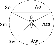
When the slippage velocity is 1, the critical water holdup can be analyzed by the Vedapuri model (1997). Figure 3 is the sketch map of oil-water flow:
Figure 3. Sketch map of the wetted perimeter in the three-phase segregated oil-water flow
The water fraction of the mixture layer ηwm can be expressed as:
$\eta_{w m}=\frac{Q_{w t}}{Q_{w t}+Q_{o t}} \times 100 \%=\frac{\gamma-\sin \gamma}{\beta+\gamma-\sin \beta-\sin \gamma}$ (38)
$S_{o}=\frac{D}{2} \cdot \beta \quad S_{w}=\frac{D}{2} \cdot \gamma S_{m}=\frac{D}{2} \cdot(2 \pi-\beta-\gamma)$ (39)
$\left\{\begin{array}{l}{A_{o}=\frac{D^{2}}{8}(\beta-\sin \beta)} \\ {A_{w}=\frac{D^{2}}{8}(\gamma-\sin \gamma)} \\ {A_{m}=\frac{D^{2}}{8}(2 \pi-\beta-\gamma+\sin \beta+\sin \gamma)}\end{array}\right.$ (40)
Substitute equations (39) and (40) into (32):
$\left(\frac{1.44(2 \pi-\beta-\gamma)+0.08\left(\sin \frac{\beta}{2}+\sin \frac{\gamma}{2}\right)}{2 \pi-\beta-\gamma+\sin \beta+\sin \gamma}+\frac{0.08 \sin \frac{\gamma}{2}}{\gamma-\sin \gamma}\right)\left(\frac{\gamma-\sin \gamma}{\gamma}\right)^{n+1} \cdot\left(\frac{2 \pi-\beta-\gamma}{2 \pi-\beta-\gamma+\sin \beta+\sin \gamma}\right)^{n}$$=1.2^{n}\left[\frac{\rho_{o}}{\rho_{w}}+\left(1-\frac{\rho_{o}}{\rho_{w}}\right) h_{w m}\right]^{n-1} \cdot\left[\frac{\rho_{o} \mu_{w}+\left(\rho_{w} \mu_{o}-\rho_{o} \mu_{w}\right) h_{w m}}{\rho_{o} \mu_{o}+\left(\rho_{w} \mu_{o}-\rho_{o} \mu_{o}\right) h_{w m}}\right]^{n}$ (41)
where
$\eta_{w m}=\eta_{w}=\frac{\gamma-\sin \gamma}{\beta+\gamma-\sin \beta-\sin \gamma}$ (42)
Similarly, the following equation is established according to the momentum of the oil layer and the mixed layer:
$\left(\frac{1.44(2 \pi-\beta-\gamma)+0.08\left(\sin \frac{\beta}{2}+\sin \frac{\gamma}{2}\right)}{2 \pi-\beta-\gamma+\sin \beta+\sin \gamma}+\frac{0.08 \sin \frac{\beta}{2}}{\beta-\sin \beta}\right)\left(\frac{\beta-\sin \beta}{\beta}\right)^{n+1} \cdot\left(\frac{2 \pi-\beta-\gamma}{2 \pi-\beta-\gamma+\sin \beta+\sin \gamma}\right)^{n}$$=1.2^{n}\left[1+\left(\frac{\rho_{w}}{\rho_{o}}-1\right) h_{w m}\right]^{n-1} \cdot\left[\frac{\rho_{o} \mu_{w}+\left(\rho_{w} \mu_{o}-\rho_{o} \mu_{w}\right) h_{w m}}{\rho_{o} \mu_{w}+\left(\rho_{w} \mu_{w}-\rho_{o} \mu_{w}\right) h_{w m}}\right]^{n}$ (43)
3.1 Overview
The test was conducted on amulti-phase flow test equipment (Figure 4). The equipment consists of an oil tube,a water tube and a gas tube. The oil tube and water tube pump working fluid to the testsystem. The testsystem is composed of a water inlet system, an oil inlet system, atest section and a measuring system.
1-Water meter; 2-Filter; 3-Stabilizer; 4-Presure gauge; 5-Flow 6-Control center;7-Fast valve; 8-Differential pressure ga9-Test section pressure gauge
Figure 4. Multi-phase flow test equipment
3.2 Test fluids
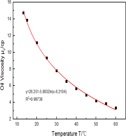
3.2.1 White oil viscosity
The oil viscosity was measured with a Brookfield DV3TLV digital viscometer and a Thermosel heater. Based on the results shown in Figure 5, the relationship between oil viscosity and temperature is obtained:
$\mu_{o}=26.251-5.8032 \ln (T-6.2104)$
Figure 5. Viscosity-temperature curve of the white oil
3.2.2 White oil density
The density of white oil varies little as temperature changes.Under the normal temperature (25oC), the white oil density is 0.857g/ml or 857kg/m3.
3.2.3 Water viscosity
Figure 6 shows the viscosity-temperature curve of the water. The relationship between water viscosity and temperature is obtained by the following formula.
$\mu_{w}=2.5059-0.4876 \ln (T+2.2805)$
Figure 6. Viscosity-temperature curve of the water
3.3 Test procedures
The test device for the oil-water two-phase flow is a closed loop. The oil and water are stored in separate tanks and pumped to the mixing tank. The oil-water ratio in the tank is adjusted to control the inlet water fraction, and to homogenize the mixture. The oil-water mixture is then pumped through the regulator and flow meters to the 9.2m-long transparent plexiglass test section. Finally, the mixture is pumped back to the mixing tankvia the gas-liquid separator for further circulation. The central control system monitors the temperature, liquid level and stirring device in the mixing tank, as well as the pressure, temperature, pressure gradient and velocity of the liquid and gas in the test section. It also controls the closing valves in the test section.
All the tests are conducted under the horizontal flow conditions at normal temperature and pressure. Table 1 specifies the parametric ranges in the test.
Table 1. Parametric ranges in the test
|
Working conditions |
|
|
Volume velocity of the mixture flow |
2, 4, 6, 8, 10, 12, 14 (m3/h); |
|
Inlet water fraction |
0, 10, 20, 30, 40, 50, 60, 80%; |
|
Test tube diameter |
40, 60 mm. |
3.4 Results and discussions
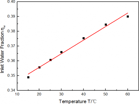
For the ST model, the test data are substituted into the Equation (22) to obtain the variation of inlet water fraction with temperature (Figure 7). In the event of low velocity, the oil and water are completely dissociated. Without considering the effect of oil-water density, it is possible to obtain the relationship between critical inlet water fraction and temperature at the oil-water slippage velocity of 0 (Uo=Uw).Figure 7 indicates that the inlet water fraction ηw is linearly correlated with temperature. When the oil and water share the same velocity, the ηw is about 35.5% at the normal temperature.
Figure 7. Inlet waterfraction variation with temperature
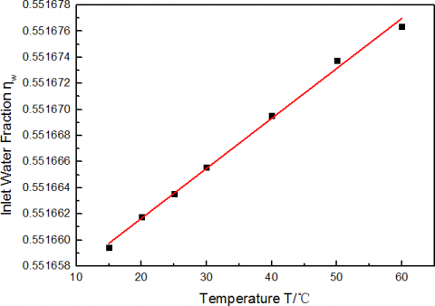
Figure 8. Inlet water fraction variation with temperature
For the three-phase segregated flow model, n=0.2 in turbulent flow. The variation in inlet water fraction ηw with temperature is obtained through the following steps: combine Equations (41) and (42), substitute n=0.2 to the combined equation, and apply the constraint that 1.2Uw=1.2Uo=Um. As shown in Figure 8, when 1.2Uw=1.2Uo=Um, the temperature has little impact on the critical inlet water fraction. At 25°C (β=2.8826, γ=3.1867), the critical inlet water fraction is about 55.17%.
There are many possible flow patterns for the oil-water flow in a horizontal pipe. According to the flow pattern maps
prepared by Arirachakam et al. (1989) and Angeli and Hewitt et al. (2000), the flow pattern (the ST) is independent of the inlet water fraction when the velocity of the mixture is less than 0.5 m/s; however, the flow pattern (the ST&MI) will become correlated with the inlet water fraction when the mixture velocity falls between 0.5m/s and 1 m/s.
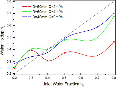
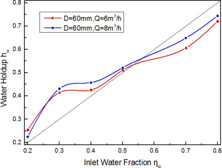
Figures 9 and 10 illustrate the variations of water holdup with inlet water fraction for the ST and the ST&MI, respectively. For the ST (Figure 9), the inlet water fraction grows slightly from 35.5% at the mixture velocity of 2m3/h to 39.5% at the mixture velocity of 4m3/h, when the water holdup hw is equal to inlet water fraction ηw. For the ST&MI (Figure 10), the inlet water fraction is about 55% when the water holdup hw is equal to inlet water fraction ηw. The water holdup results obtained from the test are in good agreement with the predicted results. The two figures demonstrate that the water holdup hw is approximately equal to the inlet water fraction ηw when the inlet water fraction reaches the critical inlet water fraction, indicating that the water holdup prediction of the no-slip oil-water flow water is well grounded.
Figure 9. Waterholdup variation with water fraction in the ST
Figure 10. Waterholdup variation with waterfraction in the ST&MI
The oil-water two-phase flow patterns could be classified into two categories: the segregated flows (ST; ST&MI) and dispersed flows (Do/w&w; O/w; Dw/o&Do/w; W/o). In the dispersed flows, the oil and water are expected to be fully mixed and the oil-water slippage velocity reaches zero. Therefore, only the ST and ST&MI are taken into account in this research.
The author puts forward a water holdup prediction model for the no-slip oil-water two-phase flow. The predicted results are proved to be true and accurate. Through further analysis of the test data, it is found that the critical inlet water fraction is about 35.5% in the ST model, and 55.17% in the three- phase segregated flow model, provided that Uo=Uw. The test results also indicate that the water holdup hw is approximately equal to the inlet water fraction ηw when the inlet water fraction reaches the critical inlet water fraction.
|
A |
the cross-sectional area of the pipe, m 2 ; |
|
S |
Sthe wetted perimeter, m ; |
|
D |
the hydraulic diameter, m ; |
|
t |
the shear stress, N / m2 ; |
|
a |
theinclination angle of the pipe; |
|
U |
the in-situ velocity, m / s ; |
|
f |
the friction coefficient; |
|
m |
the dynamic viscosity, cp ; |
|
R |
thepipe radius, m ; |
|
hw |
the waterfraction, %; |
|
hwm |
the water fractionof the mixture layer, %; |
|
Q |
the volume velocity, m3 / s ; |
|
$Q_{T}$ |
the volume velocity of the total flow, m3 / s ’ |
|
$U_{S W i n p u t}$ |
the input surface velocity of the water layer, m / s ; |
|
$U_{\text {SOinput}}$ |
the input surface velocity of the oil layer, m / s ; |
|
$U_{S W}$ |
the surface velocity of the water layer, m / s ; |
|
$U_{S O}$ |
the surface velocity of the oil layer, m /s ;
|
|
$U_{S M}$ |
the surface velocity of the mixture layer, m / s ; |
|
$h_{w}$ |
the water holdup, %. |
|
Subscripts |
|
|
o |
The oil layer |
|
w |
The water layer |
|
m |
The mixture layer |
|
i |
The oil-water interface |
|
i1 |
The water-mixture interface |
|
i2 |
The mixture-oil interface |
[1] Yan D.F., Zhang J.J., Yang X.H. (1993). Pipe Flow Characteristics of Crude Oil Water Dispersion System and Its Application in Drag Reduction, Petroleum University Publishing House, Shandong, pp. 120-135.
[2] Russel T.W.F., Hodgson G.W., Goviver G.W. (1959).Horizontal pipelines flow of mixture of oil and water,Can. J. Chem., Vol. 37, No. 1, pp. 9-17. DOI:10.1002/cjce. 5450370104
[3] Charles M.E., Goviver G.W., Hodgson W. (1961).The horizontal pipeline flow of equal density oil-water mixture, Can. J. Chem., Vol. 39, No. 1, pp. 27-36.DOI: 10.1002/cjce.5450390106
[4] Guzhov A., Grishin A.D., Medredev V.F., Medredeva O.P. (1973). Emulsion formation during the flow of two liquids in a pipe, Neft Khoz., No. 8, pp. 58-61.
[5] Malinowsky M.S. (1975). An experiment study of oilwater and air-oil-water flowing mixtures in horizontal pipes, MS Thesis, U. Of Tulsa.
[6] Oglesby K.D. (1979). An experiment study on the effect of oil viscosity, mixture, velocity and water fraction on horizontal oil-water flow, MS Thesis, U.Of Tulsa.
[7] Martinez A.E. (1983). The flow of oil-water mixtures in horizontal pipes, MS Thesis, U. Of Tulsa.
[8] Arirachakarn S., Oglesby K.D., Brill J.P. (1989). Ananalysis of oil/water flow phenomena in horizontalpipes, SPE 18836. DOI: 10.2118/18836-MS
[9] Trallero J.L. (1995). Oil-water flow patterns in horizontal pipes, Ph.D Dissertation, U. Of Tulsa.
[10] Trallero J.L., Brill J.P. (1996). A study of oil-water flow patterns in horizontal pipes, SPE 36609. DOI:10.2118/36609-PA
[11] Nadler M., Mewes D. (1997). Flow induced emulsification in the flow of two immiscible liquids in horizontal pipes, Int. J. Multiphase. Flow, Vol. 23, No.1, pp. 55-68. DOI: 10.1016/S0301-9322(96)00055-9
[12] Angeli P., Hewitt G.F. (1998). Pressure gradient in horizontal liquid-liquid flows, Int. J. Multiphase Flow 24, pp. 1183-1203. DOI: 10.1016/S0301-9322(98)00006-8
[13] Shi H., Jepson W.P. (1999). The Effect of surfactants on flow characteristics in oil/water flows in largediameter horizontal pipelines, Multiphase, pp. 181-199.
[14] Angeli P., Hewitt G.F. (2000). Flow structure in horizontal oil water flow, Int. J. Multiph. Flow 26, pp.1117-1147. DOI: 10.1016/S0301-9322(99)00081-6
[15] Chen J., Sun H.Y., Liang Z.P., Yan D.F. (2000). Flow pattern in oil-water two phase horizontal pipe flow,Oil & Gas Storage and Transportation, Vol. 12, No. 1,pp. 27-31. DOI: 10.3969/j.issn.1000-8241-D.2000.12.009
[16] Chen J. (2001). Study on oil-water two phase pipe flow, MS Thesis, University of Petroleum, Beijing,China.
[17] Chen J., Yu D., Yan D.F. (2003). Flow pattern translation in oil-water two phase flow, Research and Development of Hydrodynamics, Vol. 3, pp. 355-364.DOI: 10.3969/j.issn.1000-4874.2003.03.018
[18] Shi H. (2001). A study of oil-water flows in large diameter horizontal pipelines, Ph.D. Dissertation OhioU.
[19] Yao H.Y., Gong J. (2004). An experimental investigation on flow patterns and pressure gradient of heavy oil-water flows in horizontal pipes, The 3rd Int. Symp. On Multiphase, Non-Newtonian and Reacting Flow, Sep.10-12, Hangzhou, China.
[20] Yao H.Y. (2006). Experiment research on oil-water pipeflows, Ph.D. Dissertation, China University of Petroleum, Beijing.
[21] Al-Wahaibi T., Angeli P. (2007). Transition between stratified and non-stratified horizontal oil-water flows,part I: stability analysis, Chemical Engineering Science, Vol. 62, No. 11, pp. 2915-2928. DOI:10.1016/j.ces. 2007.01.024
[22] Al-Wahaibi T., Smith M., Angeli P. (2007). Transition between stratified and non-stratified horizontal oilwater flows, part II: mechanism of drop formation,Chemical Engineering Science, Vol. 62, No. 11, pp.2929-2940. DOI: 10.1016/j.ces.2007.01.036
[23] Al-Wahaibi T., Angeli P. (2011). Experimental study on interfacial waves in stratified horizontal oil-water flow, Int J of Multiphase Flow, Vol. 37, No. 8, pp.930-940. DOI:10.1016/j.ijmultiphaseflow.2011.04.003
[24] Al-Wahaibi T., Yusuf N., Al-Wahaibi Y., et al. (2012).Experimental study on the transition between stratified and non-stratified horizontal oil-water flow, Int J of Multiphase Flow, Vol. 38, No. 1, pp. 126-135. DOI:10.1016/ j.ijmultiphaseflow.2011.08.007
[25] Castro M., Rodriguez O. (2014). Flow pattern and pressure drop in horizontal viscous oil-water flows,10th International Conference on Heat Transfer, Fluid Mechanics and Thermodynamics.
[26] Al-Sarkhi A., Pereyra E., Mantilla I., Avila C. (2017).Dimensionless oil-water stratified to non-stratified flow pattern transition, Journal of Petroleum Science & Engineering, Vol. 3, pp. 284-291. DOI: 10.1016/j.petrol.2017.01.016
[27] Taitel Y., Dukler A.E. (1976). A model for prediction flow regime transitions in horizontal and near horizontal gas-liquid flows, AIChE J., Vol. 22, No. 1,pp. 47-55. DOI: 10.1002/aic.690220105
[28] Brauner N., Moalem M.D. (1992). Flow pattern transitions in two-phase liquid-liquid flow in horizontal tubes, Int. J. Multiphase Flow, Vol. 18, No.1, pp. 123-140. DOI: 10.1016/0301-9322(92)90010-E
[29] Vedapuri W., Jepson P. (1997). A segregated flow model to predict water layer thickness in oil-water flows in horizontal and slightly inclined pipelines,BHR Group 1997, Multiphase 97, pp. 75-105.
[30] Zeiny E., Farhadi M., Sedighi K. (2017). Numerical investigation of the simultaneous influence of swirling flow and obstacles on plate in impinging jet,International Journal of Heat and Technology, Vol.35, No. 1, pp. 59-66. DOI: 10.18280/ijht.350108
[31] Lei Y., Liao R.Q., Li M.X., Li Y., Luo W. (2017).Modified Mukherjee-brill prediction model of pressure gradient for multiphase flow in wells,International Journal of Heat and Technology, Vol.35, No. 1, pp. 103-108. DOI: 10.18280/ijht.350114