Radiation effects on Williamson nanofluid flow over a heated surface with magnetohydrodynamics

We consider a steady two dimensional flow of an incompressible MHD Williamson nanofluid over a horizontal heated surface. Where x and y- axis are taken along horizontal and vertical direction respectively, so that nanofluids confined to y>0. The plate is stretched along x-axis with the velocity $a{{x}^{n}}$, where a>0 is stretching parameter and n is the stretching index. It is assumed that the surface is heated due to convection of hot fluid below the surface. A space varying magnetic field $B(0,B(x),0)$ is applied along the transverse direction of the flow. The fluid is assumed to be slightly conducting, so that the magnetic Reynolds number is much less that unity and hence the induced magnetic field is negligible in comparison to the applied magnetic field. The general transport equations for nanofluid are given by Buongiorno [29]

div V=0,      (1)

$\rho \frac{dV}{dt}=divS+\rho b,$      (2)

$\rho c\left( \frac{\partial T}{\partial t}+V.\nabla T \right)=\nabla .k\nabla T+{{\rho }_{p}}{{c}_{p}}\left( {{D}_{B}}\nabla \varphi .\nabla T+{{D}_{T}}\frac{\nabla T.\nabla T.}{{{T}_{\infty }}} \right),$      (3)

$\frac{\partial C}{\partial t}+V.\nabla C=\nabla .\left( {{D}_{B}}\nabla C+{{D}_{T}}\frac{\nabla T}{{{T}_{\infty }}} \right),$         (4)

where in steady state the velocity vector is given by V(u(x,y), v(x,y),0), $\rho $ is nanofluid density, ${{\rho }_{p}}$ is nanoparticle density, S is Cauchy stress tensor, b is body force vector, c is the heat capacity of nanofluid, c_p is heat capacity of nanoparticles, T  is temperature, k is nanofluid thermal conductivity, D_B is Brownian diffusion coefficient, C is nanoparticle volumetric fraction, D_T is thermophoretic diffusion coefficient and ${{T}_{\infty }}$ is ambient fluid temperature. For Williamson fluid model Cauchy stress tensor S is defined in (Dapra [30]) as

$S=-pI+\tau ,$      (5)

$\tau =\left( {{\mu }_{\infty }}+\frac{\left( {{\mu }_{0}}-{{\mu }_{\infty }} \right)}{1-\Gamma \dot{\gamma }} \right){{A}_{1}},$       (6)

In above equations, $\tau $ is extra stress tensor, ${{\mu }_{0}}$ is limiting viscosity at zero shear rate and ${{\mu }_{\infty }}$ is limiting viscosity at infinite shear rate, $\Gamma >0$ is a time constant, A₁ is the first Rivlin-Erickson tensor and $\dot{\gamma }$ is defined as

$\dot{\gamma }=\sqrt{\frac{1}{2}\pi },$          (7)

where $\pi =trace(A_{1}^{2})$

Here, we considered the case for which ${{\mu }_{\infty }}=0$ and $\Gamma \dot{\gamma }<1.$ Thus equation (6) can be written as  

$\tau =\left( \frac{{{\mu }_{0}}}{1-\Gamma \dot{\gamma }} \right){{A}_{1}},$          (8)

or by using binomial expansion we get

$\tau ={{\mu }_{0}}\left( 1+\Gamma \dot{\gamma } \right){{A}_{1}},$          (9)

The interaction of magnetic field and velocity will give rise to the Lorentz force JxB defined in equation (10), in which J is the current density and $\sigma $ is the electrical conductivity. In the absence of electric field E = 0.

$J=\sigma \left( E+V\times B \right)$      (10)

Since we have considered the steady state velocity so all the derivatives w.r.t are zero. Making use of equations (5), (9) and (10) in equations (1)–(4) two dimensional boundary layer equations governing the flow are given by

$\frac{\partial u}{\partial x}+\frac{\partial v}{\partial y}=0,$         (11)

$u\frac{\partial u}{\partial x}+v\frac{\partial u}{\partial y}=\nu \frac{{{\partial }^{2}}u}{\partial {{y}^{2}}}+\sqrt{2}\nu \Gamma \frac{\partial u}{\partial y}\frac{{{\partial }^{2}}u}{\partial {{y}^{2}}}-\frac{\sigma {{B}^{2}}(x)u}{\rho },$       (12)

$u\frac{\partial T}{\partial x}+v\frac{\partial T}{\partial y}=\alpha \frac{{{\partial }^{2}}T}{\partial {{y}^{2}}}\,+\frac{{{\rho }_{p}}{{c}_{p}}}{\rho c}\left( {{D}_{B}}\frac{\partial C}{\partial y}\frac{\partial T}{\partial y}+\frac{{{D}_{T}}}{{{T}_{\infty }}}{{\left( \frac{\partial T}{\partial y} \right)}^{2}} \right)-\frac{1}{{{\rho }_{p}}{{c}_{p}}}\frac{\partial {{q}_{r}}}{\partial y}+\frac{{{Q}^{*}}}{{{\rho }_{p}}{{c}_{p}}}\left( T-{{T}_{\infty }} \right),$.    (13)

$u\frac{\partial C}{\partial x}+v\frac{\partial C}{\partial y}={{D}_{B}}\frac{{{\partial }^{2}}C}{\partial {{y}^{2}}}+\frac{{{D}_{T}}}{{{T}_{\infty }}}\frac{{{\partial }^{2}}T}{\partial {{y}^{2}}},$       (14)

where u(x,y) and v(x,y) are horizontal and vertical components of velocity, $\nu $ is kinematic viscosity and $\alpha $ is nanofluid thermal diffusivity. The magnetic field is chosen as $B(x)={{B}_{0}}\sqrt{{{x}^{n-1}}}$. The corresponding boundary conditions to the flow problem are

$u={{U}_{w}}=a{{x}^{n}};$  v = 0; $-k\frac{\partial T}{\partial y}=h\left( {{T}_{f}}-T \right),$ $C={{C}_{w}}$ 

at  y =0, $u\to 0;$  $T={{T}_{\infty }}$; $C={{C}_{\infty }}$  as $y\to \infty $          (15)

Using Rosseland approximation for radiation, the radiative heat flux is simplified as,

${{q}_{r}}=-\frac{4{{\sigma }^{*}}}{3{{k}^{*}}}\frac{\partial {{T}^{4}}}{\partial y}$        (16)

where σ* is Stefan–Boltzmann constant and k* the mean absorption coefficient. The temperature differences within the flow are assumed to be small enough so that T⁴ may be expressed as a linear function of temperature T using a truncated Taylor series about the free stream temperature ${{T}_{\infty }}$, and neglecting the higher order terms we get,

${{T}^{4}}\simeq 4TT_{\infty }^{3}-3T_{\infty }^{3}$          (17)

Substituting (16) and (17) in (13), we have

$\begin{align}  & u\frac{\partial T}{\partial x}+v\frac{\partial T}{\partial y}=\alpha \frac{{{\partial }^{2}}T}{\partial {{y}^{2}}}+\frac{{{\rho }_{p}}{{c}_{p}}}{\rho c}\left( {{D}_{B}}\frac{\partial C}{\partial y}\frac{\partial T}{\partial y}+\frac{{{D}_{T}}}{{{T}_{\infty }}}{{\left( \frac{\partial T}{\partial y} \right)}^{2}} \right) \\ & \,\,\,\,\,\,\,\,\,\,\,\,\,\,\,\,-\frac{16{{\sigma }^{*}}T_{\infty }^{3}}{3{{k}^{*}}{{\rho }_{p}}{{c}_{p}}}\frac{{{\partial }^{2}}T}{\partial {{y}^{2}}}+\frac{{{Q}^{*}}}{{{\rho }_{p}}{{c}_{p}}}\left( T-{{T}_{\infty }} \right), \\\end{align}$      (18)

In boundary conditions k is thermal conductivity, T_f is the temperature of the hot fluid and h is the convective heat transfer coefficient. Introducing the following transformations in above equations

$u=a{{x}^{n}}{f}'(\eta )$, $v=-\sqrt{\frac{a(n+1)\nu {{x}^{n-1}}}{2}}\left( f(\eta )+\frac{n-1}{n+1}\eta {f}'(\eta ) \right)$,$\eta =\sqrt{\frac{a(n+1){{x}^{n-1}}}{2\nu }},\,\,\,\theta =\frac{T-{{T}_{\infty }}}{{{T}_{w}}-{{T}_{\infty }}},\,\,\,\phi =\frac{C-{{C}_{\infty }}}{{{C}_{w}}-{{C}_{\infty }}}$        (19)

With the help of above transformations, equation (11) is identically satisfied and equations (12) (14) and (18) along with boundary conditions (15) take the following form

$\begin{align}  & {f}'''(\eta )-\frac{2n}{n+1}{{{{f}'}}^{2}}(\eta )+f(\eta ){f}''(\eta )\,+\lambda {f}''(\eta ){f}'''(\eta ) \\ & \,\,\,\,\,\,\,\,\,\,\,\,\,\,\,\,\,\,\,\,\,\,\,\,\,\,\,\,\,\,\,\,\,\,\,\,\,\,\,\,\,\,\,\,\,\,\,\,\,\,\,\,\,\,\,\,\,\,\,\,\,\,\,\,\,\,\,\,\,\,\,\,\,\,\,\,\,\,\,-M{f}'(\eta )=0, \\\end{align}$         (20)

$\begin{align}  & \left( 1+R \right){\theta }''(\eta )+\Pr f(\eta ){\theta }'(\eta )+\Pr Q\theta (\eta ) \\ & \,\,\,\,\,\,\,\,\,\,\,\,\,\,\,\,\,\,\,\,\,\,\,\,\,\,\,\,\,\,+\frac{Nc}{Le}{\phi }'(\eta ){\theta }'(\eta )+\frac{Nc}{LeNbt}{{{{\theta }'}}^{2}}(\eta )=0, \\\end{align}$          (21)

${\phi }''(\eta )+Scf(\eta ){\phi }'(\eta )+\frac{1}{Nbt}{\theta }''(\eta )=0$        (22)

Mathematically, Schmidt number Sc can be written as

$Sc=\frac{\upsilon }{{{D}_{B}}}=\frac{\alpha }{{{D}_{B}}}\frac{\upsilon }{\alpha }=Le.\Pr $          (23)

With the help of equation (23), equation (22) can be written as

${\phi }''(\eta )+Le\Pr f(\eta ){\phi }'(\eta )+\frac{1}{Nbt}{\theta }''(\eta )=0$         (24)

The corresponding boundary conditions are

$f=0,\,\,{f}'=1,\,\,{\theta }'=-Bi\left( 1-\theta  \right),\,\,\phi =1$at $\eta =0$         (25)

${f}'=0,$   $\theta =0,$     $\phi =0$     as     $\eta \to \infty $.      

Since we are interested in the study of heat transfer enhancement, so it is better to introduce the effects of thermal diffusivity in nanoparticle equation with the help of Le and Pr. Also it will enhance the coupling effects of heat and nanoparticle equation. Finally, equations (17), (18) and (21) form the non-dimensional system of equation with corresponding boundary equations given in (22). For $\lambda =0$, problem reduces to the one for Newtonian nanofluid and for D_B = D_T = 0 in equation (13), heat equation reduces to the classical boundary layer heat equation in the absence of viscous dissipation. Physical quantities of interest for the present study are skin-friction coefficient, reduced Nusselt number Nu and local Sherwood number Sh.

$Nu=\frac{-x}{{{T}_{w}}-{{T}_{\infty }}}{{\left( \frac{\partial T}{\partial y} \right)}_{y=0}}$, $Sh=\frac{-x}{{{C}_{w}}-{{C}_{\infty }}}{{\left( \frac{\partial C}{\partial y} \right)}_{y=0}}$         (26)

or by introducing the transformations (16), we get

$\frac{Nu}{\sqrt{{{\operatorname{Re}}_{x}}}}=-\sqrt{\frac{n+1}{2}}{\theta }'(0),$ $\frac{Sh}{\sqrt{{{\operatorname{Re}}_{x}}}}=-\sqrt{\frac{n+1}{2}}{\phi }'(0),$          (27)

where

${{\operatorname{Re}}_{_{x}}}=\frac{{{U}_{w}}x}{\upsilon }$ is local Reynolds number,

$\lambda =\Gamma \sqrt{\frac{{{a}^{3}}(n+1){{x}^{3n-1}}}{\nu }}$ (Non Newtonian Williamson parameter),

$\Pr =\frac{\upsilon }{\alpha }$(Prandtl number = momentum diffusivity/nanofluid thermal diffusivity),

$R=\frac{4{{\sigma }^{*}}T_{\infty }^{3}}{k{{k}^{*}}}$(Radiation parameter)

${{Q}^{*}}=\frac{Q}{{{\rho }_{p}}{{c}_{p}}a}$ (Heat source parameter)

$Le=\frac{\alpha }{{{D}_{B}}}$(Lewis number = nanofluid thermal diffusivity/Brownian diffusivity),

$Sc=\frac{\upsilon }{{{D}_{B}}}$ (Schmidt number = momentum diffusivity / Brownian diffusivity),

$M=\frac{2\sigma B_{0}^{2}}{\rho a(n+1)}$ (Magnetic field parameter),

$Nc=\frac{{{\rho }_{p}}{{c}_{p}}}{\rho c}\left( {{C}_{w}}-{{C}_{\infty }} \right)$ (Heat capacities ratio = nanoparticles heat capacity/nanofluid heat capacity),

$Nbt=\frac{{{D}_{B}}{{T}_{\infty }}\left( {{C}_{w}}-{{C}_{\infty }} \right)}{{{D}_{T}}\left( {{T}_{w}}-{{T}_{\infty }} \right)}$ (Diffusivity ratio = Brownian diffusivity /thermophoretic diffusivity),

$\frac{Bi}{\sqrt{{{\operatorname{Re}}_{x}}}}=\frac{hx}{k}\sqrt{\frac{2}{n+1}}$ (Biot number).

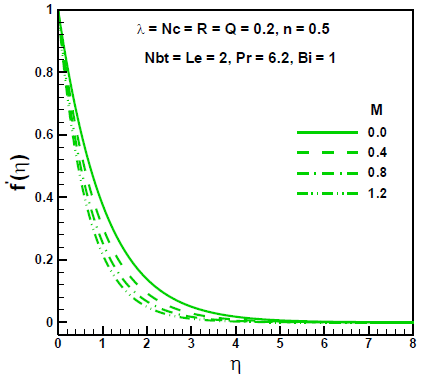
In order to investigate the physical representation of the problem, the numerical values of velocity $\left( {f}'(\eta ) \right)$, temperature $\left( \theta (\eta ) \right)$ and concentration $\left( \phi (\eta ) \right)$ have been computed for resultant principal parameters as the magnetic field parameter M, non-Newtonian Williamson parameter $\lambda $, stretching index parameter n, Biot parameter Bi, heat source parameter Q, radiation parameter R, Lewis number Le, heat capacities ratio Nc and diffusivity ratio Nbt respectively. In order to test the accuracy of the present method, our results are compared with those of Rana and Bhargava [9], Cortell [13], Zaimi et al. [14], Khan and Pop [8], Wang [15] and Gorla and Sidawi [16] (for reduced cases) and noticed that there is an excellent agreement, as shown in tables 1 and 2. Throughout the calculations, the parametric values are fixed to be M = 1.0, n = 0.5, $\lambda =Nc=R=Q=0.2$, Nbt = Le = 2.0, Pr = 6.2, Bi = 1.0, unless otherwise indicated.

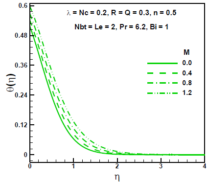
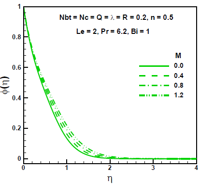
Figure 1 is drawn to examine the impact of magnetic field parameter M on the nanofluid velocity. It is observed that, the velocity profile decrease with increase in magnetic field parameter. Equation (10) involves the cross product of velocity vector and magnetic field vector, it will give rise to Lorentz force which is perpendicular to the velocity vector and magnetic field vector. This force will act as a resistive force to the fluid flow which will ultimately slow down the fluid velocity. It is also clear that the momentum boundary layer thickness decreases with increase in magnetic field parameter M. Figs. 2 and 3 demonstrate the effect of magnetic field parameter on nanofluid temperature and nanofluid concentration profile when other parameters are kept constant. Temperature profile increases with the increase in magnetic field parameter M (Fig. 2). Nanofluid contains the nano-sized particles whose motion is affected by the applied magnetic field. These particles act as the energy carrier to the fluid causing the increase in nanofluid temperature. Magnetic field is zero, when no external magnetic field is applied. We can also see that thermal boundary layer is increasing with the increase in magnetic field parameter. Concentration boundary layer increases with the increase in M as seen in Fig. 3. When the value of M increases it excites fluid particles motion which will diffuses quickly into the neighboring fluid layers due to the enhanced Brownian motion.

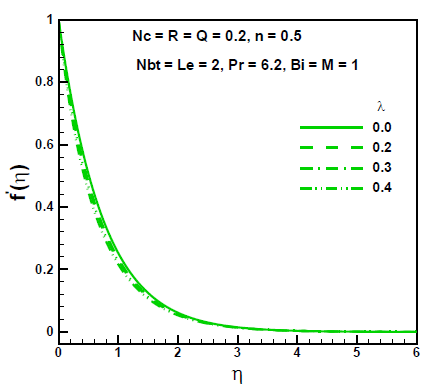
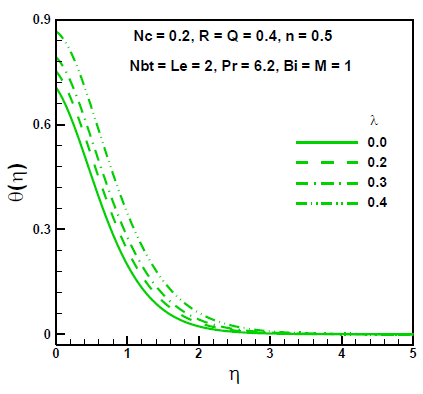
Figures 4 and 5 illustrate the nanofluid velocity and nanofluid temperature for different values of the Non Newtonian Williamson parameter$\lambda $. It is found that the velocity decreases as the Non Newtonian Williamson parameter increases (Fig. 4). From Fig. 5, it is observed that temperature profile increases with an increase in the Non Newtonian Williamson parameter.

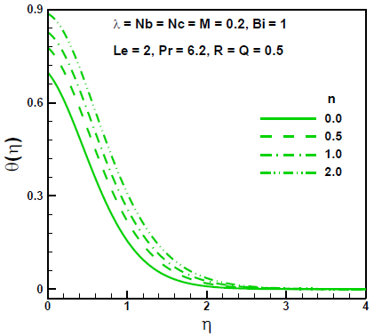
The influence of stretching index n on the velocity and temperature profiles is shown in Figs. 6 and 7 respectively. From Fig. 6, it is observed that the velocity decreases with the increasing stretching index parameter. Fig. 7 shows that temperature profiles increases with the increasing values of stretching index parameter n.

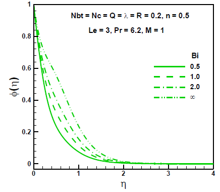
Figures 8 and 9 demonstrate the nanofluid temperature and nanofluid concentration (volumetric fraction) for different values of Biot number Bi. We can see that the temperature at wall is varying with Bi because of convective boundary conditions. When Bi approaches to infinity the temperature boundary condition at wall reduces to the case of constant wall temperature. Thus convective boundary conditions are more generalized as compare to the constant wall temperature condition. The graph also depicts that as the Bi approaches to 100, temperature attain the Biot number is the ratio of the convection at the surface to the conduction within the surface. Thus large Biot number implies stronger convection at the surface and small Biot number implies stronger conduction within the surface. Temperature graph against Bi also predicts this behaviour, the fluid temperature increases with the increase in Bi. Also thermal boundary layer increases with the increase in Bi (Fig. 8). From Fig. 9 we can also see that nanofluid concentration is increasing with the increase in Bi.

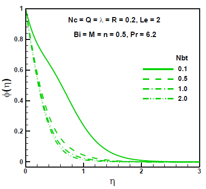
The effects of diffusivity ratio Nbt on temperature and concentration fields are presented in Figs. 10 and 11 respectively. Nbt cannot be chosen equal to zero because Nbt appears in the denominator of both Eq. (18) and (22). Buongiorno [29] defined the parameter Nbt to discuss the relative effect of Brownian diffusion to thermophoretic diffusion, we followed the same parameter. It is observed that temperature profile and thermal boundary layer decrease with increase in Nbt. when Brownian diffusivity is very large as compared to thermophoretic diffusivity, temperature profile only shows very small variation (Fig.10). Fig. 11 it is seen that concentration also decreases with increasing Nbt.

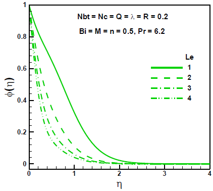
For different values of the Lewis number Le on the nanofluid temperature and nanofluid concentration are illustrated in Figs. 12 and 13 respectively. Temperature as well as concentration profile decrease with the increase in Le. Le cannot be chosen equal to zero because Le appears in the denominator of the Eq. (18). Physically Le cannot equal to zero since it is ratio of thermal diffusivity to Brownian diffusion.

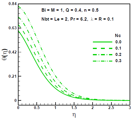
The effect of heat capacities ratio Nc on the temperature profile is studied in Fig.14. It is observed that temperature and thermal boundary layer thickness increases with the increase in Nc. If we look at the definition of Nc, it is ratio of heat capacity of nanoparticles and nanofluid. Usually the specific heat c_p of nanoparticles is less than that of base fluid be­cause typically specific heat of solid is less than that of liquids. So addition of solid particles will decrease the specific heat of base fluid, hence temperature pro­file decrease.

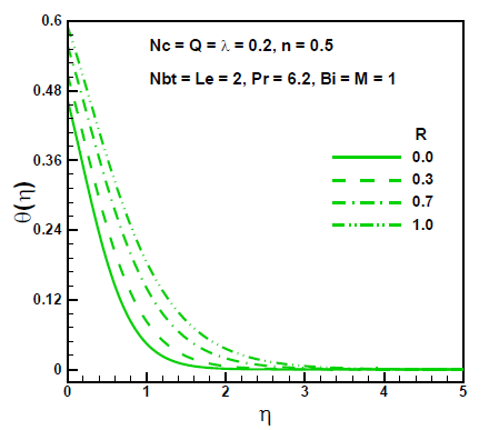
Figure 15 displays the nanofluid temperature distribution for different values of radiation parameter R. The consequence is stable for all distances into the boundary layer and validates the advantage of employing thermal radiation in nano-scale-materials dispensation processes. Through growing radiation temperature in the nanofluid is significantly intensified. R represents the comparative contribution of thermal radiation heat transfer to thermal conduction heat transfer. Subsequently thermal radiation augments the thermal diffusivity of the nanofluid, for increasing values of R heat will be added to the regime and temperatures will be increased.

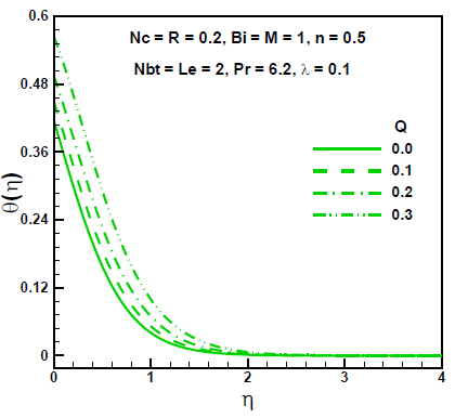
For different values of the heat source parameter Q on the nanofluid temperature distribution is displayed in Fig. 16. It is noticed that, heat generation parameter enhances the temperature leading to an increase in the thickness of the thermal boundary layer.

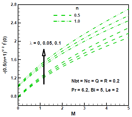
The variations of skin friction coefficient versus magnetic field parameter M is plotted in Fig.17 for different values of non-Newtonian Williamson parameter $\lambda $ in presence of stretching index number n while other parameters are kept fixed. It is evident from the Fig. 17 that the skin friction factor increases with increasing the values of non-Newtonian Williamson parameter, stretching index parameter and magnetic field parameter. Generally speaking, the effects of the magnetic field are to increase the skin friction factor and reduce the thickness of the hydrodynamic boundary layer.

Figures 18 (a) and (b) are demonstrated to show the influence of various parameters on the Nusselt number. In particularly, the simultaneous effects of magnetic field parameter, Biot number Bi and diffusivity ratio Nbt are shown in Fig. 18(a). It is observed that an increase in magnetic field parameter and diffusivity ratio causes the rate of heat transfer to decrease, on the contrary Nusselt number increases with increasing Biot number. The effects of heat generation, heat capacities ratio and radiation parameter on Nusselt number is studied in Fig. 18(b).  From this figure it is noticed that the rate of heat transfer decreases with increasing heat generation, radiation and heat capacities parameter.

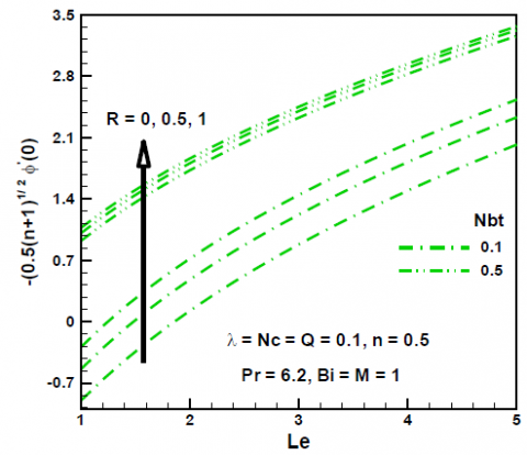
Figure 19 depicts the variation of Sherwood number with respect to the Lewis number Le for different values of radiation parameter R and diffusivity ratio Nbt. From this figure, one may observe that the rate of mass transfer increases with increasing the values of radiation parameter and diffusivity ratio.

Table 4 presents the numerical values of the skin friction coefficient, the reduced Nusselt number and reduced Sherwood number for nanofluids for various values of the non-Newtonian Williamson parameter $\lambda $, magnetic field parameter M, radiation parameter R, heat generation parameter Q, heat capacities ratio Nc, diffusivity ratio Nbt, and Biot number Bi.

It is seen from the table that the values of skin friction coefficient increases with increasing the values of non-Newtonian Williamson parameter and magnetic field parameter. It is also observed that the magnitude of heat transfer rate at the wall decreases with increasing the values of the non-Newtonian Williamson parameter, magnetic field parameter, radiation parameter, heat generation and heat capacities ratio. On the contrary it increases with increasing the values of diffusivity ratio and Biot number. It is also seen from the table 4 that the rate of mass transfer increases with an increase in the magnetic field parameter, radiation parameter, heat generation, heat capacities ratio and diffusivity ratio. On the other hand, increasing the values of non-Newtonian Williamson parameter and Biot number results in reducing rate of mass transfer.

Table 1. Comparison of $\left( -{\theta }'\left( 0 \right) \right)$ for  $\Pr $ and $n$ values when $Nc=Q=M=R=\lambda =0,\,\,Bi\to \infty $

Table 2. Comparison of Nusselt number $\left( -{\theta }'\left( 0 \right) \right)$ when $\lambda =Nc=M=Q=R=0,Bi\to \infty $ and $n=1$

1.png

Figure 1. Effects of M on dimensionless velocity

2.png

Figure 2. Effects of M on dimensionless temperature

3.png

Figure 3. Effects of M on dimensionless concentration

4.png

Figure 4. Effects of λ on dimensionless velocity

5.png

Figure 5. Effects of λ on dimensionless temperature

6.png

Figure 6. Effects of n on dimensionless velocity

7.png

Figure 7. Effects of n on dimensionless temperature

8.png

Figure 8. Effects of Bi on dimensionless temperature

9.png

Figure 9. Effects of Bi on dimensionless concentration

10.png

Figure 10. Effects of Nbt on dimensionless temperature

11.png

Figure 11. Effects of Nbt on dimensionless concentration

12.png

Figure 12. Effects of Le on dimensionless temperature

13.png

Figure 13. Effects of Le on dimensionless concentration

14.png

Figure 14. Effects of Nc on dimensionless temperature

15.png

Figure 15. Effects of R on dimensionless temperature

16.png

Figure 16. Effects of Q on dimensionless temperature

17.png

Figure 17. Effects of M, λ and n on skin friction coefficient

18.png

Figure 18. Effects of M, Nb, Bi, Q, R and Nc on Nusselt number

19.png

Figure 19. Effects of M, λ and n on Sherwood number